Vue lecture
Kubernetes 1.36 restores a lost guarantee for database backups
It’s 2 a.m., and you’re restoring a PostgreSQL cluster from last night’s backup. Its data directory lives on one PersistentVolumeClaim and its write-ahead log on another, a common split for I/O isolation. Every volume snapshot reported success. The pods come back. Then Postgres refuses to start because the WAL on one volume references pages that were never captured in the data files on the other. The backup wasn’t corrupted in transit. It was inconsistent the moment it was taken.
If you run stateful workloads on Kubernetes, this failure mode has been silently lurking in your backups for years. It has nothing to do with your backup tool crashing, and everything to do with a guarantee you gave up when you moved off traditional storage.
The consistency group you lost on the way to Kubernetes
Enterprise storage arrays solved this problem decades ago with a feature called a consistency group. You told the array which LUNs belonged to the same application, and when you snapshotted the group, the array froze them all at the same instant. Every volume captured the same point in time. Restores were coherent by construction.
“The backup wasn’t corrupted in transit. It was inconsistent the moment it was taken.”
That guarantee didn’t survive the move to cloud native. The Container Storage Interface (CSI) standardized snapshots around a single object, the VolumeSnapshot, scoped to a single PersistentVolumeClaim (PVC). One PVC, one snapshot. For a stateless service with one volume, that model is fine. For anything that spreads its state across multiple volumes (a database with separate data and log disks, a sharded datastore, most real applications), the per-PVC model can’t tell which volumes belong together.
As teams migrated off proprietary SANs and virtualization stacks onto Kubernetes-native storage, they gained enormous flexibility but lost the consistency group. Most never notice since the gap only shows up at restore time after an incident, when it is far too late to do anything about it.

How individual PVC snapshots break
When protecting a multi-volume application, backup tools enumerate the PVCs and issue a VolumeSnapshot for each one, in sequence. Snapshot volume A, volume B, then volume C.
Each snapshot is individually crash-consistent, equivalent to pulling the power cord on that one volume. But they are not consistent with one another. Between snapshotting A and snapshotting B, the application keeps writing. A transaction can land in the log on volume B that references data never captured on volume A, because A was frozen a few hundred milliseconds earlier. The busier the application and the more volumes involved, the wider the inconsistency window.
“The result is a set of snapshots that each looks healthy and collectively describes a state that never existed.”
The result is a set of snapshots that each looks healthy and collectively describes a state that never existed. You can quiesce the application to close the window (freeze I/O, flush buffers, snapshot, unfreeze), but at production scale, freezing a busy database for the duration of a multi-volume snapshot is exactly the disruption backups are supposed to avoid.
VolumeGroupSnapshot: consistency groups as a Kubernetes API
VolumeGroupSnapshot is the missing primitive, and as of Kubernetes v1.36 (May 2026), it is generally available. It brings the consistency group back as a first-class, vendor-neutral Kubernetes API rather than a proprietary array feature.
The model has three objects. A VolumeGroupSnapshotClass, defined by an administrator, describes how group snapshots are created for a given CSI driver. A VolumeGroupSnapshot is the user’s request, and it carries a label selector that picks out every PVC belonging to the application. A VolumeGroupSnapshotContent tracks the provisioned result. Under the hood, the CSI driver takes one atomic, point-in-time snapshot across every selected volume: a real consistency group, with no application quiescence required, provided the underlying storage supports it.
“Under the hood, the CSI driver takes one atomic, point-in-time snapshot across every selected volume.”
The label selector is the important design choice. You don’t enumerate volumes; you describe them. A selector like `app=postgres` picks up the data and logs PVCs together, and the group boundary is expressed in Kubernetes terms that survive adding or resizing volumes over time.
Wiring it into backup: what changes
An API that produces consistent snapshots only helps if your backup workflow uses it. When I implemented VolumeGroupSnapshot support in Velero, the CNCF project that has become the de facto standard for Kubernetes backup and restore, the core change was replacing “iterate over PVCs and snapshot each” with “group the PVCs that belong together, snapshot the group as one operation, then track the per-volume members for restore.”
That last part matters. A group snapshot fans back out into individual volume snapshots, one per member, so restore still rehydrates each PVC independently, but now every member shares a single point in time. Velero was among the first backup projects to build directly on the upstream VolumeGroupSnapshot API, rather than a proprietary grouping scheme, so the consistency guarantee rides on a standard the whole ecosystem shares instead of a format locked to one tool.
Individual snapshots vs. group snapshots: which to use
This is not a wholesale replacement. Individual PVC snapshots remain the right tool for single-volume workloads and for volumes that are genuinely independent, since snapshotting those as a group buys you nothing and adds coordination overhead. Reach for VolumeGroupSnapshot when correctness depends on multiple volumes sharing a point in time.
A quick decision guide:
- One volume, or several fully independent volumes: individual VolumeSnapshots.
- Multiple volumes with cross-volume write ordering (data plus WAL, data plus index): VolumeGroupSnapshot.
- Unsure whether a skewed or partial restore would corrupt the application? Treat it as a group.
Day 2 notes
A few things to check before relying on this in production. Group snapshot support is per CSI driver: the API is standard, but the driver has to implement it, and adoption is still spreading. A growing set of CSI drivers implement it (Ceph CSI among them), so check the driver’s release notes for upstream VolumeGroupSnapshot support, and create the VolumeGroupSnapshotClass before needing it. The atomicity guarantee is only as strong as the storage backend behind the driver, so validate it by restoring, not by reading success statuses. Audit existing backups now: by protecting multi-volume applications with per-PVC snapshots today, you likely have inconsistent restore points that have never been tested under a real failure.
“With VolumeGroupSnapshot now GA and backup tooling adopting it upstream, multi-volume backups on Kubernetes are finally consistent by construction, not by luck.”
The broader arc is that Kubernetes storage is catching up to what enterprise arrays offered for years, but as an open standard rather than a capability locked to one vendor’s hardware. Consistency groups were one of the last missing pieces. With VolumeGroupSnapshot now GA and backup tooling adopting it upstream, multi-volume backups on Kubernetes are finally consistent by construction, not by luck.
The post Kubernetes 1.36 restores a lost guarantee for database backups appeared first on The New Stack.
[In preview] Public Preview: Agentless migration of on-premises SMB file shares to Azure Files (SMB)
Introducing Amazon EBS Volume Clones across AWS accounts
Last year, we introduced Volume Clones of Amazon Elastic Block Store (Amazon EBS), a new capability that lets you create instant point-in-time copies of your EBS volumes within the same Availability Zone.
Today, we are extending Volume Clones with cross-account copy, so you can create copies of your EBS volumes into other AWS accounts and optionally re-encrypt them with an AWS Key Management Service (AWS KMS) key in the target account.
With this new feature, you can use your latest application data to develop, test, and experiment in a secondary environment, while protecting and isolating the information in the production environment. For example, you can create copies of a production environment to refresh test and development environments set up in separate accounts with the desired EBS encryption.
Copy EBS volumes across AWS accounts in action
To create a copy of an EBS volume across accounts, the owners of the volume can first grant the target account access to their volume in AWS Resource Access Manager (RAM), which provides a way to share resources across AWS accounts or within an AWS Organization. Then, from the target account, they can locate the volume they have access to create a copy of it.
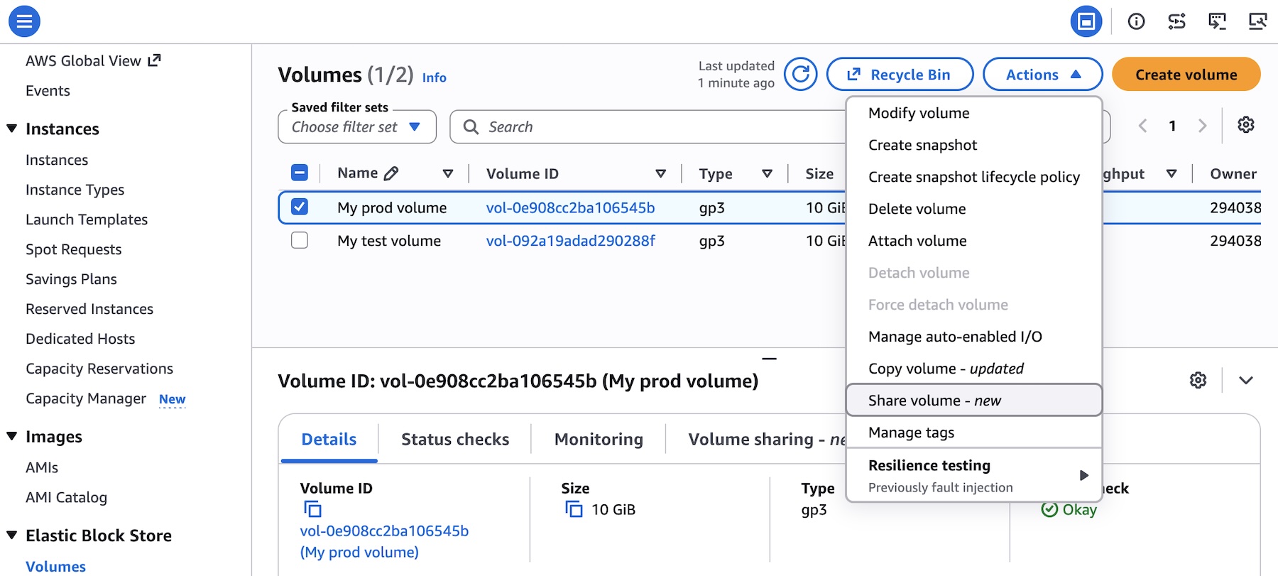
To get started, choose Share volume for the volume you want to share with the target account in the Amazon EBS console.

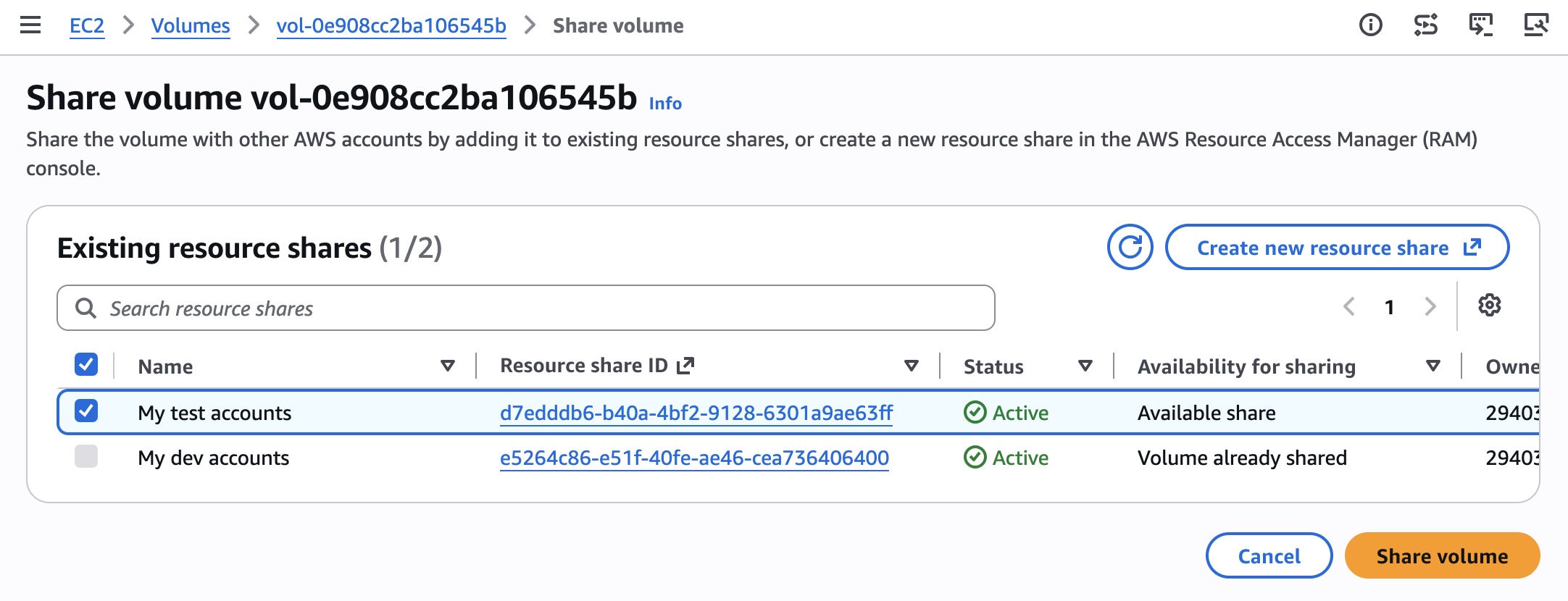
Share the volume with other AWS accounts by adding it to existing resource shares, or create a new resource share in the AWS RAM console. For more details, refer to the AWS RAM User Guide.

You can now see confirmation that the volume has been shared in the Volume sharing tab of the volume detail page.

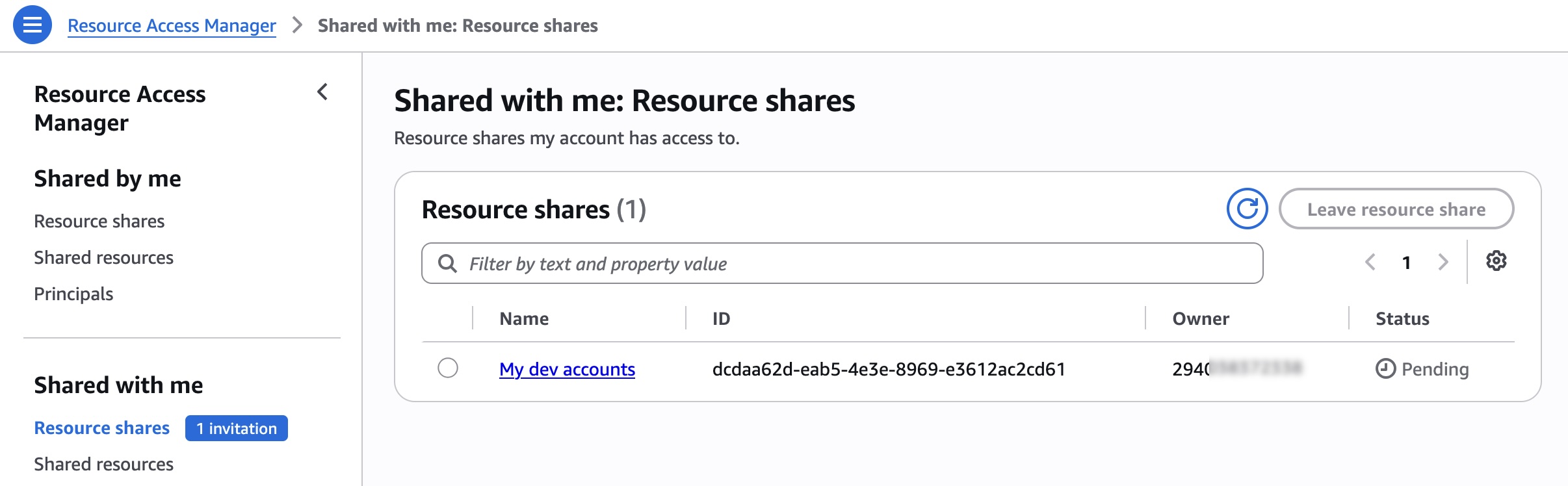
A target account must accept the resource share on the RAM console.

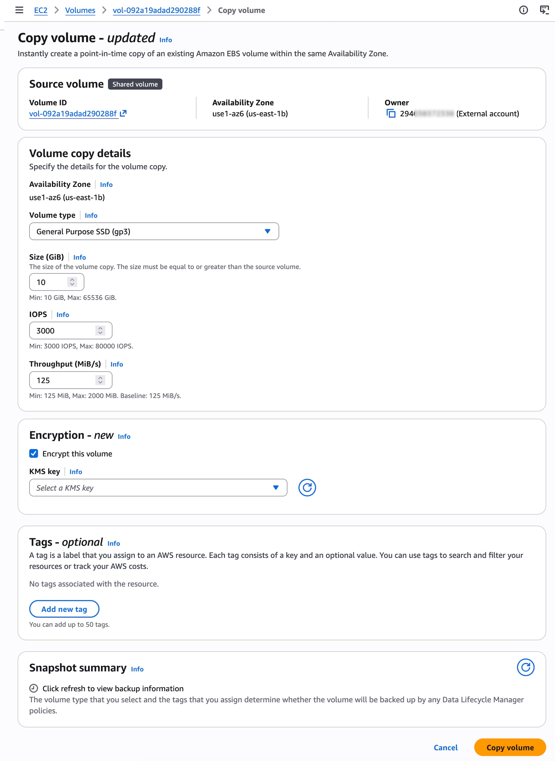
Once they accept the resource share, they can see the volumes in the EBS volume page of the target account. Choose Copy volume for any shared volume.

To share and copy EBS volumes across AWS accounts programmatically, including calling APIs and searching documentation, try the AWS MCP Server and plugins with your preferred AI coding tool. To learn more, visit the Amazon EBS User Guide.
Things to know
Let me share some important technical details that I think you’ll find useful.
- Encryption: You can share unencrypted volumes and volumes encrypted with a customer managed key (CMK). Volumes encrypted with the default AWS managed key (AMK) cannot be shared. When copying a shared volume encrypted with a CMK, the CMK must also be shared with the target account. You can specify a different CMK to re-encrypt the copy in the target account.
- Monitoring: You can monitor
SharedVolumeCopyInitiatedthrough AWS CloudTrail event in your account. You will also receive events in Amazon EventBridge at the start of the copy operation when the state of the copied volume isinitializing, and at the end of the operation when the state of the copied volume changes tocompleted. You can see the shared volume ID, consuming account ID, and event time. - Pricing: Once a copy is initiated, you’ll pay a one-time fee based on your volume size, charged to the account where the copy will reside. There’s no cost for sharing EBS volumes through AWS RAM. The copied volume will incur regular EBS volume charges upon creation.
- Availability Zone: The volume copy must be created in the same Availability Zone as the source volume. Use Availability Zone IDs (such as
use1-az1) to identify the same physical location across accounts.
Now available
Cross-account volume clones for Amazon EBS are available in all AWS Regions that support Amazon EBS Volume Clones. For Regional availability and a future roadmap, visit the AWS Capabilities by Region.
Give this feature a try in the Amazon EC2 console today and send feedback to AWS re:Post for Amazon EBS or through your usual AWS Support contacts.
— Channy
[Launched] Generally Available: User-bound user delegation SAS for Azure Storage
[Launched] Generally Available: Azure Developer CLI (azd) Extension Framework
[In preview] Public Preview: Per-disk resiliency for Azure VMs
[Launched] Generally Available: Workload identity support for Azure Files CSI driver (SMB) in Azure
When AI agent traces become application data

Say a test starts failing and a developer hands it to a coding agent. It digs into the relevant files, runs the test suite, changes two files, then runs targeted validation. The task view shows the files it touched, the commands it ran, what results those commands returned, and the diff it landed on.
Before accepting the patch, the developer reviews that activity. A teammate might reopen the same run later to see why the code changed. The team building the agent can compare thousands of runs to see whether a model or prompt update improved test success or just added more tool calls and cost.
That record needs somewhere to live. Developers and reviewers want a durable version of the run whenever they need it. Engineering wants the same execution data aggregated across runs, because the agent’s behavior is nondeterministic and shifts over time.
“For many agentic products, that record turns out to be application data with a telemetry-shaped workload.”
For many agentic products, that record turns out to be application data with a telemetry-shaped workload. That’s the combination that changes the storage decision.
When a trace becomes product data
Not every agent trace counts as application data. An internal diagnostic trace that can be sampled, expired, or discarded is still telemetry. That boundary can exist within the same trace, where raw diagnostic fields remain internal and the fields needed to reconstruct the user’s task move into product state.
The boundary moves once your product has to retrieve, display, or retain a durable execution record. A developer, for example, might need to see which files an agent inspected, or a reviewer might need to check which commands ran and whether the tests passed.
This doesn’t require exposing a model’s private chain of thought. The product can instead render a projection of observable execution, showing model invocations, tool calls, file reads, command results, errors, timing, and state transitions. That record lets users verify the result and decide how much they want to trust it. In some workflows, it also becomes an audit record, which changes its access and retention requirements.
“Internal diagnostic fields don’t automatically belong in the product view just because they came from the same run.”
Once that execution record becomes product state, it must follow your application’s access model. Code, prompts, retrieved documents, tool arguments, and command output may carry tenant or user data, so the application must enforce the same authorization boundaries when storing and retrieving them. Internal diagnostic fields don’t automatically belong in the product view just because they came from the same run.
Why one agent run produces so much data
Pull request volume scales with the number of patches submitted for review, and issue volume scales with the number of development tasks. Both are just counting units of work at the workflow boundary.
Agent traces scale differently, depending on the execution graph within each task. One request to fix a failing test can trigger multiple model calls, file reads, searches, command executions, test retries, and branches before the agent ever proposes a patch. Each of those steps can produce its own span or event.
OpenTelemetry GenAI semantic conventions, still in development, define separate span types for model inference, tool execution, and retrieval. What gets captured depends on the span type and content-capture policy. Inference spans may carry model identifiers, token usage, and opt-in input and output messages, while tool-execution spans may carry opt-in arguments and results.
The span count tracks what the agent actually does inside each unit of work. If you add a new tool, a retry policy, or a branch, the data volume can increase even though the number of completed tasks hasn’t changed.
“If you add a new tool, a retry policy, or a branch, the data volume can increase even though the number of completed tasks hasn’t changed.”
This same fan-out also shows up outside coding agents. In a case study, Laminar reported more than 500,000 browser events per day. A browser-agent session could run for more than 30 minutes and generate hundreds of thousands of DOM diff events. Laminar used those events to reconstruct a video-like replay of what the agent saw.
Whether the agent writes code or navigates a browser, the same data serves two different purposes. One person loads one trace to understand a single run, and the engineering team scans many traces to find patterns. That combination of point retrieval and cohort analysis gives this data its unusual shape.
Why agent trace data behaves like telemetry
Most records in an agent trace are written once rather than updated. A model invocation or tool result describes an event that has already happened. Scores, annotations, and run status may change later, but teams can store those mutable fields separately or record the changes as new events.
The records also carry high-cardinality dimensions such as model version, prompt template, tool name, session ID, user ID, and outcome. Their value only shows up in context. On its own, an isolated tool-call span doesn’t say much, but a full trajectory can explain a failed run, while a cohort can reveal a regression.
The same dataset therefore serves several distinct readers:
| Consumer | Read pattern | Example |
|---|---|---|
| Product interface | Point lookup | Load one coding-agent run for a developer or reviewer |
| Evaluation pipeline | Cohort scan | Compare test success, latency, and cost across agent versions |
| Platform team | Time-window aggregation | Group errors and latency by model, tool or deployment |
A primary application database can serve all three patterns at modest scale, but that changes when wide scans and high-cardinality aggregations start competing with product reads and writes on the critical path.
Outgrowing the primary database
There is no universal event-count threshold for moving traces out of the primary database. The decision shows up in the workload.
The first signal is contention, where ingestion or retention work starts consuming enough I/O and CPU to affect transactional operations. Next comes analytical friction, where evaluations and debugging queries need to scan long time ranges or join large trace tables, and stop meeting your team’s latency target. Eventually, teams resort to forced sampling, discarding traces to protect the application database, even though the product or an audit process requires the complete record.
Langfuse documented both contention and analytical friction as it scaled its open-source platform for LLM observability, evaluation, and prompt management. It experienced Postgres IOPS exhaustion during ingestion and prompt API latency reaching seven seconds under heavy load. Langfuse moved its tracing data from Postgres to ClickHouse, while keeping transactional and latency-sensitive paths isolated.
The store is only half the decision
The database move solved one class of problem, but the original data model created another. Langfuse initially carried separate trace, observation, and score tables into its analytical architecture. Updates required deduplication and cross-table analysis, adding join cost.
“The store is only half the decision. The analytical storage engine addressed the workload, and a data model reduced cross-table work.”
Later, Langfuse collapsed those records into a wide, mostly immutable observations table, with one row per model call, tool execution, or agent step. Initial table loads for large datasets went from seconds to milliseconds, and dashboard load times for large projects improved by at least 10 times over longer time ranges.
Langfuse needed both changes. The analytical storage engine addressed the workload, and a data model reduced cross-table work.
How to choose a storage pattern
Start with the reads your product must support, then choose the simplest architecture that meets those requirements.
At modest volume, keeping traces in the primary database avoids another operational boundary. As analytical contention grows, the application can send trace events to a dedicated analytical store while keeping mutable business records in its transactional database.
Some applications need both systems to share data. A Postgres-backed product might keep users, permissions, and workflow state in Postgres while sending agent events to ClickHouse for analytical queries. If relevant application data already lives in Postgres, change data capture can replicate it into the analytical path.
Start with who reads the trace
Who depends on the record and how they query it matters more than whether a trace looks like a log or a pull request.
If your product needs to reconstruct a durable record of a single run and the engineering team needs to compare behavior across thousands of runs, the trace has become application data with a telemetry-like storage workload.
Map the point lookups and cross-run scans before choosing a store. If both are product requirements, design for both from the first trace you retain.
The post When AI agent traces become application data appeared first on The New Stack.
[Launched] Generally Available: Live Resize for Shared Premium SSD v2 and Ultra Data Disks
[In preview] Public Preview: Migrate from AWS FSx for Windows File Server to Azure Files with Azure Storage Mover
[In preview] Public Preview: Support for SMB Opportunistic Locking (Oplocks) configuration
[Launched] Generally Available: Encryption in Transit for Azure Files NFS Shares in Azure Kubernetes Service (AKS)
[In preview] Public Preview: Advanced platform metrics in Azure Monitor
[Launched] Generally Available: Microsoft Entra ID-based access for Azure Blob Storage SFTP
[In preview] Public Preview: Instant Access via application consistent restore points
[Launched] Public Preview: Azure Storage Mover now supports migration from Google Cloud Storage (GCS)
[Launched] Generally Available: Client-side data integrity protections in Azure Blob Storage
[In preview] Generally Available: Azure NetApp Files migration assistant
Amazon S3 annotations: attach rich, queryable context directly to your objects
Today, we’re announcing a new metadata capability for Amazon Simple Storage Service (Amazon S3) called annotations, enabling you to attach rich, large-scale business context directly to your objects. You can store up to 1,000 named annotations per object, each up to 1 MB in size, totaling up to 1 GB per object, in flexible formats like JSON, XML, YAML, or plain text. You can modify or delete an annotation at any time, without re-writing your objects, making it easy to keep your object context current.
Organizations are building AI agents and autonomous workflows that need to find, understand, and act on data without human intervention. To support these agentic workflows, you need metadata that can evolve alongside the data, scale to petabytes of objects, and remain queryable without expensive retrieval.
With S3 annotations, you can store context such as AI-generated transcripts, content ratings, or technical specifications directly alongside your objects. Your context moves automatically with the object during copy, replication, and cross-region transfers, and S3 removes it when you delete the object. When you enable S3 Metadata, annotations automatically flow into fully managed annotation tables that you can query with Amazon Athena and other analytics engines.
Common use cases
Annotations solve complex metadata challenges across industries:
- Media & Entertainment: Track transcripts, content moderation results, subtitle files, and licensing metadata as separate annotations on video assets, eliminating the need to synchronize metadata across multiple media asset management systems.
- Financial Services: Attach AI-generated investment summaries and sentiment analysis to research documents, enabling autonomous research agents to discover relevant datasets through natural-language queries without maintaining separate metadata databases.
- Life Sciences: Annotate clinical trial data with regulatory status, patient cohort details, and approval chains, making compliance audits faster while keeping full context accessible for archived data in Amazon S3 Glacier storage classes without retrieval charges.
How annotations address metadata challenges
Amazon S3 already supports several ways to describe your objects. System-defined metadata captures properties like size and storage class. Object tags support operational tasks like access control and lifecycle management. User-defined metadata lets you add small amounts of custom information at upload time.
While these capabilities work well for their intended purposes, they have limitations when you need to attach much richer context without building and maintaining separate metadata systems. Annotations address these needs by providing metadata capabilities at a fundamentally different scale and flexibility, offering mutable, queryable context per object compared to 10 immutable tags or 2 KB of headers.
| Capability | Max size | Mutable? | Best for |
| System-defined metadata | Fixed | No | Object properties (size, storage class, creation time) |
| User-defined metadata | 2 KB | No (set at upload) | Small custom key-value pairs |
| Object tags | 10 tags, 128/256 characters per key/value | Yes | Access control, lifecycle rules, cost allocation |
| Annotations | 1 GB (1,000 × 1 MB) | Yes | Rich business context (JSON, XML, YAML, plain text) |
Today, metadata describing S3 objects often lives in separate databases or sidecar files, requiring complex synchronization workflows that can exceed data storage costs. When you enable S3 Metadata annotation tables, this context becomes queryable at scale through Amazon Athena. AI agents can discover your data through natural language with the S3 Tables MCP server, which provides a standardized interface for AI models to query your annotations. You can query annotations for objects in any storage class, without restoring the objects or paying retrieval charges.
Getting started with annotations
To start using annotations, make sure your AWS Identity and Access Management (IAM) policy or bucket policy grants permissions for the s3:PutObjectAnnotation and s3:GetObjectAnnotation actions. You can then add annotations to any existing or new S3 object using the PutObjectAnnotation API.
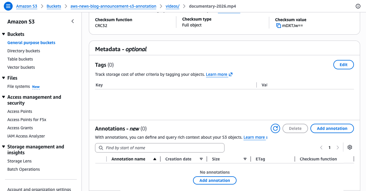
For example, a media company can attach technical specifications and AI-produced summaries to a video asset using the AWS Command Line Interface (AWS CLI):
# Create a JSON file with technical metadata
cat > mediainfo.json << 'EOF'
{"codec":"H.265","resolution":"3840x2160","audio_tracks":8,"frame_rate":29.97}
EOF
# Attach it as an annotation
aws s3api put-object-annotation \
--bucket my-media-bucket \
--key videos/documentary-2026.mp4 \
--annotation-name mediainfo \
--annotation-payload ./mediainfo.json
# Attach a plain-text AI-generated summary as a separate annotation
echo "A 90-minute nature documentary covering wildlife migration patterns across three continents, featuring aerial footage and underwater sequences. Languages: English, Spanish, Portuguese." > ai_summary.txt
aws s3api put-object-annotation \
--bucket my-media-bucket \
--key videos/documentary-2026.mp4 \
--annotation-name ai_summary \
--annotation-payload ./ai_summary.txt
These commands attach two separate annotations to the same video object. The mediainfo annotation stores structured technical specifications as JSON, while the ai_summary annotation stores a text description. Each annotation is identified by a unique name, and you can read and modify each one independently. With unique names for each annotation, you can use different annotations to support multiple concurrent enrichment workflows, for example, one team adding technical metadata while another team adds content classifications, without interfering with each other.
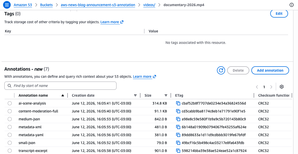
Retrieve a specific annotation using the GetObjectAnnotation API:
aws s3api get-object-annotation \
--bucket my-media-bucket \
--key videos/documentary-2026.mp4 \
--annotation-name mediainfo \
./mediainfo-output.json
To see all annotations attached to an object, use the ListObjectAnnotations API:
aws s3api list-object-annotations \
--bucket my-media-bucket \
--key videos/documentary-2026.mp4
When you no longer need a specific annotation, remove it using the DeleteObjectAnnotation API:
aws s3api delete-object-annotation \
--bucket my-media-bucket \
--key videos/documentary-2026.mp4 \
--annotation-name mediainfo
You can update an existing annotation at any time by calling PutObjectAnnotation again with the same annotation name. For large objects uploaded using multipart upload, attach annotations after completing the multipart upload using the PutObjectAnnotation API.
Querying annotations at scale with S3 Metadata tables
Attaching annotations to individual objects is useful, but the real power comes when you query across all your annotations at scale. When you enable S3 Metadata annotation tables on your bucket, S3 automatically indexes your annotations into a fully managed Apache Iceberg table, called an annotation table. You can query annotation tables with Amazon Athena or any Iceberg-compatible engine.
To enable annotation tables, use the S3 console or the CreateBucketMetadataConfiguration API. The following example creates a new metadata configuration with annotation tables enabled while keeping journal tables for change tracking and disabling the live inventory table:
{
"JournalTableConfiguration": {
"RecordExpiration": { "Expiration": "DISABLED" }
},
"InventoryTableConfiguration": { "ConfigurationState": "DISABLED" },
"AnnotationTableConfiguration": {
"ConfigurationState": "ENABLED",
"Role": "arn:aws:iam::123456789012:role/S3MetadataAnnotationRole"
}
}
This configuration tells S3 to automatically capture all your annotations in a queryable table. Once applied, any annotation you attach to objects in this bucket will appear in the table within approximately one hour.
If the bucket already has a metadata configuration, use the UpdateBucketMetadataAnnotationTableConfiguration API:
aws s3api update-bucket-metadata-annotation-table-configuration \
--bucket my-media-bucket \
--annotation-table-configuration '{"ConfigurationState":"ENABLED","Role":"arn:aws:iam::123456789012:role/S3MetadataAnnotationRole"}'
Once enabled, your annotations automatically flow into the annotation table. Journal tables update in near real time, while annotation tables refresh within an hour. Unlike traditional metadata tables that require predefined schemas, annotation tables automatically adapt to any JSON, XML, or YAML structure you write. Each annotation becomes a row in the table with its content stored in a text_value column, letting you query across all annotations without schema migrations.
If you enable annotation tables on a bucket that already has annotated objects, S3 automatically backfills existing annotations into the table. The backfill process runs in the background and can take several hours to days depending on the number of objects.
For example, to find all video assets with more than 8 audio tracks across your entire bucket using Amazon Athena:
SELECT DISTINCT bucket, object_key
FROM "s3tablescatalog/aws-s3"."b_my_media_bucket"."annotation"
WHERE name = 'mediainfo'
AND CAST(json_extract_scalar(text_value, '$.audio_tracks') AS INTEGER) > 8
This query scans the annotation table for all annotations named mediainfo, extracts the audio_tracks field from the JSON content, and returns objects where the count exceeds 8.
Or to find all objects that received new annotations in the last 24 hours through the journal table:
SELECT bucket, key, version_id, record_timestamp, annotation.name
FROM "s3tablescatalog/aws-s3"."b_my_media_bucket"."journal"
WHERE record_timestamp >= (current_date - interval '1' day)
AND annotation.name IS NOT NULL
AND record_type IN ('CREATE_ANNOTATION', 'DELETE_ANNOTATION')
This query uses the journal table to track annotation changes in near real time, which is ideal for building event-driven workflows that respond to new or deleted annotations.
You can also use natural language to search objects by their annotations using agents in Amazon SageMaker Unified Studio or any IDE with the S3 Tables MCP server. For example, asking “find all PG-rated movies with Spanish subtitles from 2023” returns results in seconds instead of the hours it would take querying multiple disconnected systems.
Get started today
You can start using Amazon S3 annotations today in all AWS Regions, including the AWS China Regions. Annotation tables are available in all AWS Regions where S3 Metadata is available.
Whether you’re building AI agents that need to discover data autonomously, managing petabytes of media assets with complex metadata, or tracking compliance context for archived datasets, annotations give you the scale and flexibility to attach rich metadata directly to your objects without managing separate systems.
Annotation storage is always billed at S3 Standard rates, even if the parent object is in S3 Glacier or another storage class. For full pricing details, visit the Amazon S3 pricing page.
To learn more and get started, visit the Amazon S3 Metadata overview page and the Amazon S3 documentation. Send feedback to AWS re:Post for S3 or through your usual AWS Support contacts.
Daniel Abib