The surge in AI development has created unprecedented demand for compute capacity around the globe. This can have negative implications for data processing and pipelines with Apache Spark. Whether you are managing your own Spark infrastructure or using a managed service, you can face availability constraints. However, a significant advantage of using Google’s Managed Service for Apache Spark is the availability of flexible VMs, which provide a targeted mechanism to adopt a dynamic, resource-agnostic philosophy and ensure your pipelines remain operational, even during regional or zonal capacity stockouts.

Understanding capacity stockouts

Capacity stockouts occur when demand for a specific machine family (such as N2 or N2D) exceeds available capacity in a target zone or region. For time-sensitive analytics pipelines, rigid single-VM requirements transform standard provisioning into a single point of failure which can result in cluster creation delays, failed executions, and potentially compromised business SLAs.

Flexible VMs

Flexible VMs fundamentally overhaul how a Managed Spark cluster requests compute resources. Rather than binding a cluster to a rigid instance type, flexible VMs allow teams to establish an ordered list of acceptable machine families for master, primary worker, and secondary worker nodes.

Key features

• Multi-family blending: Mix nodes across diverse machine types and generations, combining Gen2 families (e.g., N2, N2D) with Gen4 families (e.g., N4, C4) in a single configuration.

• Mixed storage support: Broaden available capacity pools by allowing storage options to dynamically adapt to the underlying host family's supported disk types.

• Comprehensive cluster coverage: Apply flexible rules to primary workers, secondary (preemptible/spot) workers, and master nodes to guarantee cluster provisioning end-to-end.

Ranked configuration: A strategy for success

A successful flexible VM implementation relies on intentional ranking. By defining a clear hierarchy of options, Managed Spark clusters automatically attempt provisioning, systematically mitigating stockout risks without requiring manual intervention. To improve the availability of  suitable VMs, we recommend specifying at least two machine families in the highest priority (Rank 0) flexible VM list.

As an example, for production pipelines standardizing on n2d-standard-16 shapes, the following tiering strategy provides robust resilience against capacity constraints:

code_block

<ListValue: [StructValue([('code', 'gcloud dataproc clusters create $CLUSTER_NAME \\\r\n--num-workers=10 \\\r\n--zone="" \\\r\n--region=us-east1 \\\r\n--worker-instance-selection=\'{"machineTypes":["n2d-standard-16","n2-standard-16"],"rank":0,"diskConfig":{"bootDiskType":"pd-standard","bootDiskSizeGb":400}}\' \\\r\n--worker-instance-selection=\'{"machineTypes":["n4-standard-16","n4d-standard-16"],"rank":1,"diskConfig":{"bootDiskType":"hyperdisk-balanced","bootDiskSizeGb":400}}\' \\\r\n--worker-instance-selection=\'{"machineTypes":["c4-standard-16","c3-standard-22"],"rank":2,"diskConfig":{"bootDiskType":"hyperdisk-balanced","bootDiskSizeGb":400}}\' \\\r\n--worker-instance-selection=\'{"machineTypes":["e2-standard-16"],"rank":3, "diskConfig":{"bootDiskType":"pd-ssd","bootDiskSizeGb":400}}\' \\\r\n--master-instance-selection=\'{"machineTypes":["n4-standard-16","n4d-standard-16"],"rank":0,"diskConfig":{"bootDiskType":"hyperdisk-balanced","bootDiskSizeGb":400}}\''), ('language', ''), ('caption', <wagtail.rich_text.RichText object at 0x7fb3fbbd5a90>)])]>

For pipelines standardizing on legacy n1-standard-16 shapes, the following tiering strategy helps transition workloads toward newer, more available architectures while preserving operational stability:

Leveraging Hyperdisk Balanced

Unlocking maximum availability with flexible VMs often requires adopting modern storage architectures like Hyperdisk Balanced. Newer instance families (including N4 and C4) rely on Hyperdisk to deliver predictable performance across variable VM sizes. Starting with default IOPS and throughput settings typically provides a reliable baseline for the majority of distributed Spark jobs.

Trade-offs and key considerations

While flexible VMs  dramatically improve cluster provisioning success, aligning them with enterprise requirements involves evaluating several architectural and financial factors:

1. Resource quotas

It is no longer enough to have one specific machine (e.g., N2) quota. You need to ensure you have sufficient compute and disk quotas allocated for all specific machine types and disks (including Hyperdisk) defined in their flexible VM lists.

2. Compute flexible Committed Use Discounts (CUDs)

Traditional, resource-based CUDs are tied to specific machine families, which limits flexibility. Adopt Compute flexible Committed Use Discounts (CUDs) to apply savings across multiple VM families and regions.

3. Performance Characteristics

Performance can vary between machine generations, as well as between Local SSD and Hyperdisk. While the Managed Spark team maintains internal benchmarks for these comparisons, actual outcomes are workload-dependent. Testing your specific Spark jobs across these families is essential for understanding SLA impacts.

Additional recommendations

In addition to implementing flexible VMs, there are several other key architectural and scheduling strategies to improve resource availability and workload stability:

• AutoZone: Implement AutoZone routing to allow Managed Spark to automatically select the zone best suited to execute the job based on current capacity.

• Smaller machine shapes: Avoid high in demand, large-core shapes. Design workloads and YARN containers to utilize smaller machine shapes (such as 4, 8, or 16 cores). These smaller shapes are much easier to fulfill from the available GCE on-demand pool.

• Autoscaling: Deploy cluster autoscaling with reasonable maxInstances to manage capacity effectively for bursty or unpredictable workloads without relying on rigid, massive upfront provisioning.

• Partial cluster creation: Configure a minimum acceptable number of primary workers. This allows clusters to spin up under resource constraints and begin executing, while autoscaling can dynamically add remaining workers as resources become available.

• Establish regional fallbacks: Some regions, such as us-central1, can experience  high demand. Setting up fallbacks to other regions reduces capacity stockout risks.

Keep your Spark jobs running with flexible VMs

Managing your own Apache Spark infrastructure can be complex, especially when capacity stockouts disrupt your data processing. Utilizing a managed service like Managed Service for Apache Spark provides unique advantages — including built-in platform resilience and access to flexible VMs. By adopting a prioritized fallback strategy with flexible VMs, you can protect your workloads from regional hardware shortages and keep your critical pipelines running.

Ready to improve your Spark workload resilience? Start configuring flexible VMs for your Managed Spark clusters today.

Today, we are excited to announce enhancements to the borderless Lakehouse, our answer to how data engineers, data scientists, and increasingly, AI agents, can query governed data directly where it lives.

To reason accurately and automate complex enterprise workflows, agents and data consumers of all types need fast, unified access to an organization's complete data estate, joining customer records, transaction logs, and operational telemetry across clouds. However, modern enterprise data is rarely confined to a single location; data estates often span Amazon S3, Azure Data Lake Storage (ADLS), Google Cloud Storage, operational databases, and SaaS platforms like Salesforce, SAP, and Workday. Historically, uniting these distributed datasets required brittle ETL pipelines, duplicated storage, and prohibitive cross-cloud data transfer costs.

We introduced the borderless Lakehouse earlier this year to let organizations query and activate data in place across clouds. By adopting the Apache Iceberg REST catalog specification, we federate directly to catalogs such as Databricks Unity Catalog, AWS Glue, and Snowflake Horizon. We also introduced Partner Cross-Cloud Interconnect to establish high-bandwidth, private links to other cloud providers, lowering per-gigabyte transfer costs compared to the public internet. 

Today, we are taking multi-cloud efficiency a step further by optimizing how much data needs to be transferred across the wire in the first place.

We are excited to announce two new features to help further reduce costs of querying cross-cloud data.  First, the preview of cross-cloud caching for Lakehouse transparently accelerates cross-cloud queries in BigQuery and cuts remote transfer costs by caching frequently accessed data locally in Google Cloud. Combining standard Iceberg columnar compression with cross-cloud caching means you often only need to transfer under 5% of the data you process across clouds, which helps lower the Total Cost of Ownership (TCO) to make cross-cloud analytics and AI viable at enterprise scale. In addition, BigQuery cross-cloud connections are also available in preview to query non-Iceberg data in other clouds and accelerate workloads.

How cross-cloud caching works

Cross-cloud caching meets enterprise performance and security requirements with no knobs to turn or storage to manage to accelerate your queries. Some of the mechanisms used under the hood are:

• Sub-file block granularity: Instead of transferring entire multi-gigabyte files across clouds when a query touches only a few columns, cross-cloud caching operates at the sub-file block level for columnar formats like Apache Parquet. BigQuery caches only the specific column chunks and dictionary pages projected by the query. On a cache miss, BigQuery fetches the needed data from the remote cloud to answer the query, and saves a local copy in the cache for future queries, drastically cutting network transfer and latency on repeated workloads.

• Default encryption at rest: Cached data blocks are encrypted at rest by default using Google-managed encryption keys (GMEK) so that temporary cache storage maintains the same enterprise-grade security posture as native BigQuery storage without extra overhead.

• Tenant and regional isolation: Cache entries are strictly partitioned by project and catalog boundaries to help prevent cross-tenant data exposure. Lakehouse anchors both the local cache and query execution strictly to the configured Google Cloud region (e.g., us-east4) to support compliance with regional data residency requirements when querying remote clouds.

• Freshness checks: Multi-cloud caching often forces a trade-off between speed and freshness. To avoid stale reads, BigQuery fetches remote object metadata before using cached data to ensure the data hasn’t changed and the user still has access. Any upstream table modification prompts BigQuery to fetch new files, while unreferenced cached blocks expire automatically, delivering local query speed with single-source-of-truth accuracy.

For more details on caching mechanics, statistics counters, and regional considerations, see the Lakehouse intelligent caching documentation.

Cross-cloud caching in action

So how does this work in day-to-day operations? Consider an e-commerce team querying a 10 TiB Iceberg sales table (aws_lakehouse_catalog.sales.web_sales) in Amazon S3, federated into Lakehouse from Databricks Unity Catalog. During evening promotional drops (8:00–9:00 PM), analysts query historical transactions to identify which storefronts drive peak volume and revenue among high-intent demographics:

code_block

<ListValue: [StructValue([('code', 'SELECT w.web_name, hd.hd_buy_potential, COUNT(*) AS total_transactions, ROUND(SUM(ws.ws_sales_price), 2) AS total_sales\r\nFROM `aws_lakehouse_catalog.sales.web_sales` ws\r\n-- Joins household_demographics, time_dim (8:00-9:00 PM), and web_site.\r\nGROUP BY w.web_name, hd.hd_buy_potential;'), ('language', ''), ('caption', <wagtail.rich_text.RichText object at 0x7f09257a4190>)])]>

Initial execution: Cold columnar retrieval

On this initial cold run, the local cache is empty (cacheBytesRead: "0"). BigQuery applies partition pruning and column projection to transfer only the required Parquet byte ranges from Amazon S3 over Partner Cross-Cloud Interconnect:

code_block

<ListValue: [StructValue([('code', '{\r\n "totalBytesProcessed": "230343464114",\r\n "objectStorageStats": [\r\n{"cloudProvider": "AWS", \r\n"objectStorageBytesRead": "25834740486", \r\n"cacheBytesRead": "0"}]\r\n}'), ('language', ''), ('caption', <wagtail.rich_text.RichText object at 0x7f09257a7ad0>)])]>

• Logical data processed: BigQuery processes 214.5 GiB across the 10 TiB dataset.

• Standard Iceberg compression efficiency: BigQuery reads 24.1 GiB from S3 thanks to standard Iceberg columnar compression with Zstandard (zstd) — an 8.9:1 compression ratio. As these sub-file Parquet blocks arrive in Google Cloud, BigQuery populates the regional cache.

Follow-on exploration: Adding a dimension

In practice, analysts and agents rarely run the exact same query twice in a row. To drill deeper into fulfillment methods, the analyst modifies the query by adding the shipping method dimension (sm.sm_type):

code_block

<ListValue: [StructValue([('code', 'SELECT w.web_name, sm.sm_type, hd.hd_buy_potential, COUNT(*) AS total_transactions, ROUND(SUM(ws.ws_sales_price), 2) AS total_sales\r\nFROM `aws_lakehouse_catalog.sales.web_sales` ws\r\nJOIN `aws_lakehouse_catalog.sales.ship_mode` sm ON ws.ws_ship_mode_sk = sm.sm_ship_mode_sk\r\n-- Reuses existing joins on household_demographics, time_dim, and web_site.\r\nGROUP BY w.web_name, sm.sm_type, hd.hd_buy_potential;'), ('language', ''), ('caption', <wagtail.rich_text.RichText object at 0x7f09257a62d0>)])]>

Job statistics for this follow-on query show:

code_block

<ListValue: [StructValue([('code', '{\r\n "totalBytesProcessed": "287928766472",\r\n "objectStorageStats": [\r\n{"cloudProvider": "AWS", \r\n"objectStorageBytesRead": "1426587648", \r\n"cacheBytesRead": "25834740486"}]\r\n}'), ('language', ''), ('caption', <wagtail.rich_text.RichText object at 0x7f09257a46d0>)])]>

• 94.8% cache hit rate: BigQuery serves 24.1 GiB of previously queried columns directly from local cache.

• Granular remote retrieval: BigQuery transfers only 1.33 GiB from S3 for the new ws_ship_mode_sk column and ship_mode table.

• Sub-file flexibility: Modifying a query reuses cached column chunks and transfers only newly required bytes.

Compounding efficiency at enterprise scale

When thinking about TCO of cross-cloud queries, the top two factors to account for are:

• Compression ratio: when using default compression algorithms (Zstandard/zstd) on Iceberg, columnar data is highly compressible. If you assume that your data achieves a compression ratio of 8:1, it means every 1 TiB of logical data processed only requires ~128 GiB of data to move over the network.

• Cache hit rates: when data is retrieved from cache rather than across the network because it was recently accessed, a network transit is avoided. Assuming 80% of your data results in a cache hit it means for every 100 GiB of physical data accessed only 20 GiB moves over the network.

Taking both factors and assumptions into account, for every 1 TiB of data your organization processes, you only need to transfer ~26 GiB across the network (under 3% of total data processed). Combining this reduction with Partner Cross-Cloud Interconnect lowers TCO enough to make cross-cloud analytics and AI cost-effective at petabyte scale.

BigQuery cross-cloud connections now in preview

Alongside cross-cloud caching, the preview of BigQuery cross-cloud connections lets organizations connect BigQuery directly to open-format data in Amazon S3 and Azure Storage. 

Understanding when to use catalog federation versus cross-cloud connections is straightforward:

• BigQuery cross-cloud connections (for raw files): For standalone files (CSV, JSON, ad-hoc Parquet) without an Iceberg catalog, cross-cloud connections let you create BigQuery external tables referencing remote bucket paths directly.

• Lakehouse catalog federation (for Iceberg): For Iceberg data managed by catalogs like Databricks Unity, AWS Glue, or Snowflake Horizon, Lakehouse automatically synchronizes schemas and table snapshots to simplify the user experience and ensure users are always querying the latest data.

Cross-cloud connections serve as the modern architectural evolution by using standard BigQuery compute workers in Google Cloud regions rather than compute workers in other clouds. This approach helps unlock global region availability and provides full BigQuery feature parity — including with BigQuery AI and Gemini on remote files.

The cross-cloud caching capabilities for Lakehouse applies to data queried from BigQuery cross-cloud connections as well as Lakehouse catalog federation. To learn how to create connections and query external bucket paths, see the BigQuery cross-cloud connections setup documentation.

Operating large data pipelines requires an orchestration layer that scales smoothly as workloads expand. When your pipelines process millions of complex data points every day to feed predictive models, staying up-to-date with your technology stack is a strategic necessity.

Pine59 provides location intelligence data through data pipelines that produce analytical metrics on cadences ranging from hourly to quarterly. One of the company’s most data-intensive metrics, Daily Foot Traffic, computes data for as many as 14 million distinct locations in a single job. To handle this massive volume, Pine59’s system runs entirely on Google Cloud, with the heavy lifting in BigQuery and all of it orchestrated by Managed Service for Apache Airflow (formerly Cloud Composer) running Apache Airflow 3.

As the company’s volume of data and number of machine learning workloads scaled up, Pine59 decided to modernize its monorepo, which contains hundreds of directed acyclic graphs (DAGs). Here is a look at how that transition improved Pine59’s MLOps capabilities, developer workflow, and pipeline speed.

Proactive modernization for growth

Pine59 has long relied on a shared monorepo with code and tooling spanning multiple projects to run its metric production pipelines. As it considered its infrastructure’s future, the company wanted to help its data pipelines run faster and more reliably.

That’s why it decided to stress-test production workloads against the newly available Managed Airflow (Gen 3) architecture running Airflow 3. The initial results were unambiguous: the Gen 3 environment delivered immediate and significant processing speed, task scheduling, and overall stability improvements. Recognizing the clear potential for performance gains, Pine59 initiated a full transition to the new environment.

Orchestrating advanced MLOps

Pine59’s pipelines don’t just move data; they drive complex ML models, so a core aspect of its migration was optimizing the orchestration of its ML inference workloads.

Previously, Pine59 had used standard Kubernetes operators for these tasks. By moving to Managed Airflow (Gen 3), which features a highly optimized and abstracted infrastructure layer, the company’s engineering team refined its MLOps architecture. They did so by setting up a dedicated Google Kubernetes Engine (GKE) cluster that was specifically optimized for model inference and integrated it into the Pine59 pipelines.

This clear separation of orchestration and heavy ML execution compute allows data processing and model inference to run efficiently, showcasing Managed Airflow as a resilient, scalable backbone for enterprise MLOps.

Supporting developers with custom extensibility

Beyond infrastructure improvements, Pine59 was also able to immediately capitalize on Airflow 3’s delivery of a vastly improved developer workflow and user interface. Indeed, managing hundreds of interconnected DAGs requires excellent observability, and Pine59 found Airflow 3’s plugin authoring system remarkably easy to use.

To improve internal developer velocity, the company quickly built a number of custom plugins that it integrated directly into its new Airflow UI:

• BigQuery Auto-linkify: A tool that automatically detects internal BigQuery table references within the Airflow Logs and XCom tabs, dynamically generating direct links to BigQuery Studio for faster debugging (available as a public GitHub gist)

• DAG Run Configuration Search: A custom search form added directly to the DAG overview page. It allows Pine59 engineers to query specific key-value pairs within DAG run payloads (configs) and instantly surface matching runs. This in turn drastically reduces troubleshooting time.

In addition, the team also deployed a compatibility shim layer within its monorepo. This “compat” module dynamically abstracts logic between Airflow versions, streamlining operator migration across versions.

Faster, more reliable pipelines

For Pine59, migrating to Managed Airflow (Gen 3) with Airflow 3 has yielded clear, quantifiable results.

The most important improvement was the speed of its DAG runs. In the company’s previous setup, tasks often got stuck in a queued state during peak processing surges. With Gen 3, queue latency has dropped dramatically, allowing tasks to start running almost immediately.

Consider the comparison below of total aggregated “queued” & “running” time of more than 300 runs of the same DAG between Managed Airflow (Gen2) with Airflow 2.11 vs. Managed Airflow (Gen3) with Airflow 3.1 below. As we can readily see, the difference in queued time is significant.

Coupled with internal DAG optimizations made during the transition, the performance gains are also highly tangible. For example, the Daily Foot Traffic pipeline previously took nearly 38 minutes to complete. With the new instance, the same workload now takes less than 26 minutes —nearly 32% less processing time.

Today, Pine59 processes all its production workloads on its new Managed Airflow (Gen 3) instance. By moving to this next generation orchestration, the company improved its MLOps capabilities, equipped its developers with better tools, and built a faster, more resilient foundation for future workloads.

If your engineering team spends more time managing infrastructure than delivering value, consider a similar transition and discover how it can help you move from maintaining servers to building the future of your data and AI pipelines today.

^{Special thanks to the following contributor to this post: Alexandre Crespo-Perez}

The telecommunications industry is currently undergoing a paradigm shift, moving from traditional manual human-driven operations to fully Autonomous Network Operations. Modern networks have grown increasingly complex, heterogeneous, and large-scale, making handcrafted rules-based methods and traditional Machine Learning (ML) approaches alone insufficient to automate network operations. While ML methods can identify subtle patterns and make fine predictions from large amounts of structured data, they lack the ability to understand, reason about the data and the system it represents, and ultimately make the kind of decision a human operator would.

The growth of AI agents and their ability to reason is a promising solution to this shortcoming. However, in the same way a human operator is not capable of directly ingesting the statistical information spread across the billions of data points created in a large network, AI agents also lack the ability to operate at this scale. To address this challenge, telecommunications companies are adopting Graph Neural Networks (GNNs), a modern form of machine learning designed to operate natively on massive volumes of temporal and relational data. By integrating GNNs with AI agents, operators can combine advanced diagnostics such as root cause analysis, capacity planning, traffic forecasting, what-if simulations, and real-time anomaly detection with the reasoning power required to interpret these insights and execute justified actions. This powerful combination enables networks to safely move towards Level 5 Autonomy as defined by TM Forum, where the system operates autonomously. 

In this post, we present the three components (Data, ML, and AI) that will power Google Cloud’s Autonomous Network Operations framework.

Foundation: Digital Twin on Spanner Graph

At the heart of Google Cloud’s Autonomous Network Operations framework is the network digital twin: a highly detailed, virtual replica that continuously mirrors its living telecommunications network in real time. Rather than being a static model, it is represented as a dynamic, temporal network graph that captures the evolving state and relations of its components over time. This architectural approach allows operators to "go back" in time to train and evaluate ML models on historical data, while providing AI agents with the foundational operational knowledge required to achieve Level 5 Autonomy. By simulating the impact of proposed network changes within this digital environment, the Digital Twin establishes a critical layer of trust, enabling AI agents to confidently design future states and automatically resolve network issues.

Google Cloud’s Spanner Graph is well suited to host this digital twin:

• Scalability and Availability: Spanner Graph provides a no compromise foundation for modern applications, offering virtually unlimited scaling that grows as the network grows, along with 0-RPO/0-RTO and five 9s of availability.

• Multi-Model Support: Supports multiple data models (Relational, Graph, Vector, and Full-Text Search) in a single platform allowing developers to build complex compositions such as graph transversals combined with nearest neighbor vector search.

• Global Consistency: Spanner provides a globally consistent view of the network, simplifying system development.

The next figure illustrates a network topology with four node types: routers, interfaces (the physical ports), VPNs (L3VPN service instances), and flows (active traffic sessions). These are connected by directed edge types capturing the full network stack: physical containment (router-interface), physical links (interface-interface), control-plane peering (router-router via OSPF/iBGP), service membership (router-VPN), and traffic anchoring (flow-interface, flow-VPN).

The ML layer: Distributed Graph Flow (DGF)

To predict how a network will behave and react, the digital twin leverages an ML layer powered by Distributed Graph Flow (DGF). By training on the vast volumes of structured historical data hosted within Spanner Graph, this layer uncovers critical predictive insights that enable human operators and AI agents to manage networks proactively rather than reactively.

DGF is a recently open-sourced Python library designed to manage the entire end-to-end lifecycle of GNN modeling. Developed by Google CoreML and Google Research, it brings a decade of internal Google-scale tools and expertise directly to Google Cloud enterprise clients. To accommodate different engineering needs, the library offers high-performance, composable, low-level primitives for advanced teams, alongside a simple API for rapid development that requires no prior GNN expertise.

For instance, training and evaluate a GNN model in GraphFlow with the high level API can be as simple as writing 5 lines of code:

code_block

<ListValue: [StructValue([('code', 'import dgf\r\n\r\n# Fetch the data from Spanner Graph\r\ngraph, schema = dgf.io.read_spanner_graph(...)\r\n\r\n# Train a node attribute prediction model\r\nmodel = dgf.learning.train_node_model(graph, schema, target_column="risk_score")\r\n\r\n# Evaluate the model\r\nmodel.evaluate()\r\n# Make predictions\r\nmodel.predict(graph, seed_node_idxs=[0, 1, 2])\r\n\r\n# Save the model for later\r\nmodel.save("/tmp/model")'), ('language', ''), ('caption', <wagtail.rich_text.RichText object at 0x7fce29db6350>)])]>

The DGF provides high-level concepts that map directly to Autonomous Network Operations requirements:

Use cases

By leveraging DGF and GNNs, telcos can move from reactive maintenance to proactive prevention through several advanced use cases:

• Anomaly detection: GNNs generate node and edge embeddings that encapsulate historical patterns and current health. Any anomalous embeddings are flagged for review before they lead to service degradation.

• Root cause analysis (RCA): DGF can output specific subgraphs containing only the relevant network instances related to an incident, such as "Attach Failures" in a specific ZIP code. This allows troubleshooting agents to perform high-speed analysis without scanning the entire global network.

• Predictive maintenance: The system can predict the likelihood of device failures or edge breaks, such as "handover failures" for fast-moving equipment, enabling proactive load balancing or rerouting. Furthermore, by combining agents, remedial actions can be automated by adopting a ‘human-on-the-loop’/’human-in-the-loop’.

• What-if analysis: GNNs enable Telcos to simulate scenarios like fiber cuts,  or traffic surges or device configuration changes. By modeling topological dependencies, GNNs can predict how these local changes propagate across the entire network, allowing engineers to test resilience and evaluate mitigation strategies in a risk-free digital environment.

Scenario: Root cause analysis with GNNs and DGF

Once you have created a digital twin (example code), a straight-forward 5-step process can be used to implement Root Cause Analysis(RCA) detection using GNNs and DGF. 

1. Connect to the Digital Twin: Use the DGF Spanner Graph connector (dgf.io.read_spanner_graph) to load the network topology directly from Spanner Graph's Digital Twin into the DGF environment.

2. Train a Supervised Node (or Edge) Prediction model: Depending on the training data and objective, you will train a supervised node prediction model to predict a target node feature or an edge prediction model to predict an edge between the root cause entity node and the affected entity node. For the given sample data you will use the high-level dgf.learning.train_node_model API to train a supervised node prediction model.

3. Use the node prediction model to predict root cause node: The node prediction model can be directly used to predict the impact score on the node with the anomaly. Entity nodes affected by the anomaly with highest predicted impact score will be the top candidates for root cause.

4. Deploy to Gemini Enterprise Agent Platform (formerly Vertex AI): Export the model and host it on a Gemini Enterprise endpoint to enable scalable, low-latency predictions.

5. Real-time Inference: Make prediction calls to the inference endpoint with the anomaly date as input. The endpoint will return the predicted root cause Entity nodes. 

Get started today

The integration of GNN using Distributed Graph Flow into network operations is more than just a technical upgrade; it is a critical evolution for the telco industry. By moving towards a GNN-powered autonomous framework, operators can significantly shorten outage times, optimize capacity in real-time, and ultimately deliver a superior customer experience through improved operational efficiency. 

To start building your own intelligent network applications, check out the Distributed GraphFlow (DGF) library, which provides the essential primitives for scalable GNN training and inference. For a hands-on experience, follow our step-by-step code sample. You can also explore our recent award-winning Moonshot project on Business-aware GNN-healing networks, and dive deeper into our approach on self-optimizing autonomous networks by reviewing this whitepaper.

BigQuery now features a suite of augmented analytics Table-Valued Functions (TVFs) designed to automate complex data analysis at scale. Augmented analytics combines AI, ML and statistical methods to automate insight discovery and pattern explanation. These functions allow you to diagnose why metrics changed, uncover underlying trends and relationships across the data, and even isolate the true impact of business decisions. 

These TVFs run directly where your data lives, which helps speed up analysis and reduces the need to export data into external tools. In addition, since these functions are compact and yield structured SQL outputs, they can easily be integrated as skills for AI agents, which easily enables automated, conversational data investigation workflows. 

We are introducing six new augmented analytics functions in BigQuery, each created to address a specific analytical challenge:

As we show in the next section, these functions can be easily chained together. The output of one function, such as a detected time window, can directly parameterize the next analytical step.

A step-by-step example of chaining insights

Consider a case where there is a shift in a metric, and you need to diagnose the underlying cause and measure the business lift. 

To diagnose, we can chain ML.DETECT_CHANGE_POINTS, AI.KEY_DRIVERS and AI.CAUSAL_EFFECT using the Austin Bikeshare sample dataset (bigquery-public-data.austin_bikeshare.bikeshare_trips). This dataset contains historical trip volume and demographic data for the city’s bikesharing program. 

Step 1: Detect change points

ML.DETECT_CHANGE_POINTS automatically identifies statistically significant structural shifts or level changes in your time-series data. While this example demonstrates the analysis  in a single aggregate metric, this function is highly scalable and is capable of running across millions of individual time series. 

To find these shifts,  we run the following query across the daily baseline:

code_block

<ListValue: [StructValue([('code', "WITH daily_trips AS (\r\n SELECT\r\n TIMESTAMP_TRUNC(start_time, DAY) AS trip_day,\r\n COUNT(*) AS total_trips\r\n FROM `bigquery-public-data.austin_bikeshare.bikeshare_trips`\r\n GROUP BY 1\r\n)\r\nSELECT\r\n begin_timestamp,\r\n end_timestamp,\r\n metrics.avg AS avg_daily_trips,\r\n metrics.min AS min_daily_trips,\r\n metrics.max AS max_daily_trips,\r\n metrics.count AS duration_days\r\nFROM ML.DETECT_CHANGE_POINTS(\r\n (SELECT * FROM daily_trips),\r\n data_col => 'total_trips',\r\n timestamp_col => 'trip_day'\r\n);"), ('language', ''), ('caption', <wagtail.rich_text.RichText object at 0x7f313193db90>)])]>

The output identifies the exact time intervals where the baselines have shifted over the company’s history:

If we look at the raw daily session counts, this aligns with shifts over time. We highlight the two change points with the longest durations below:

The shift in February 2018 aligns with the day the Austin City Council passed the “Dockless Mobility Pilot Program”, to transform the transit ecosystem, integrating shared electric scooters and bikes into the public. 

Step 2: Key drivers attribution

We can input the February 2018 slice found directly to AI.KEY_DRIVERS to determine the particular factors (i.e. bike_type, subscriber_type, etc) driving the surge. AI.KEY_DRIVERS can scan through millions of rows of multi-dimensional data in seconds. 

We define the interest group as the slice of time after the shift occurs and compare it against the time period before the shift as the reference group.

code_block

<ListValue: [StructValue([('code', "WITH daily_segments AS (\r\n SELECT \r\n start_station_name,\r\n end_station_name,\r\n subscriber_type,\r\n bike_type,\r\n 1 AS trip_count,\r\n -- We use the precise breakpoint identified by Change Points\r\n IF(EXTRACT(DATE FROM start_time) >= '2018-02-11', TRUE, FALSE) AS after_shift\r\n FROM `bigquery-public-data.austin_bikeshare.bikeshare_trips`\r\n -- Equidistant ~30 day window around the event\r\n WHERE start_time BETWEEN '2018-01-12' AND '2018-03-13'\r\n)\r\nSELECT \r\n drivers,\r\n metric_interest,\r\n metric_reference,\r\n difference,\r\n relative_difference,\r\n unexpected_difference,\r\n contribution\r\nFROM AI.KEY_DRIVERS(\r\n (SELECT * FROM daily_segments),\r\n metric_col => 'trip_count',\r\n interest_label_col => 'after_shift',\r\n dimension_cols => ['start_station_name', \r\n 'end_station_name', \r\n 'subscriber_type', \r\n 'bike_type'],\r\n top_k => 10\r\n);"), ('language', ''), ('caption', <wagtail.rich_text.RichText object at 0x7f3130d38f50>)])]>

AI.KEY_DRIVERS isolates the top contributing dimension values.  Each row contains a segment, which represents a slice of data identified by a specific combination of dimension values (e.g., subscriber_type = 'UT Student' and bike_type = 'classic').

The analysis reveals that the overall trip count increased +374.7% (+40,159 trips) between the reference and interest time windows. The massive growth was overwhelmingly concentrated in U.T. Student Memberships (+7,167.1%) and trips ending at the 21st & Speedway @PCL station (+20,739.1%).

This aligns with Austin Bikeshare’s response to the Dockless Mobility Pilot Program. In early February, the bikeshare program launched a large promotional partnership with the University of Texas that offered free annual memberships to all UT students.

Step 3: Causal effect

While we know what drove the surge and when it started, we need to isolate the true return on investment over organic expectations. AI.CAUSAL_EFFECT can construct an ARIMA_PLUS counterfactual to measure what the volume would have been had the program never launched.

code_block

<ListValue: [StructValue([('code', "WITH daily_trips AS (\r\n SELECT \r\n TIMESTAMP_TRUNC(start_time, DAY) AS trip_day, \r\n COUNT(*) AS total_trips\r\n FROM `bigquery-public-data.austin_bikeshare.bikeshare_trips`\r\n -- Training on the 6-month baseline leading up to the intervention\r\n WHERE start_time BETWEEN '2017-08-11' AND '2018-04-11'\r\n GROUP BY 1\r\n)\r\nSELECT \r\n *\r\nFROM AI.CAUSAL_EFFECT(\r\n (SELECT * FROM daily_trips),\r\n data_col => 'total_trips',\r\n timestamp_col => 'trip_day',\r\n -- We inject the breakpoint found in Step 1 as our intervention\r\n intervention_timestamp => '2018-02-11 00:00:00',\r\n output_time_series => TRUE\r\n);"), ('language', ''), ('caption', <wagtail.rich_text.RichText object at 0x7f3130d3bcd0>)])]>

If we graph the predicted and actual trips per day, we can see the surge compared to the counterfactual.

If we set the output_time_series => FALSE, we can see a summary of the lift

AI.CAUSAL_EFFECT reveals that the program caused a +358% volume surge above organic baseline projections, resulting in an estimated 89,775 incremental trips (with 99.9% probability of causal effect).

Connecting augmented analytics to Conversational Analytics

Conversational Analytics lets you chat with agents about your data using natural language. All new BigQuery augmented analytical functions are now available in Conversational Analytics. Since these TVFs can execute complex analytics at BigQuery-scale in seconds, Conversational Analytics can orchestrate multi-step investigative workflows based on a given prompt. Below we show two examples:

Example 1: Chicago taxi trips

Here is an example using the Chicago Taxi Trips (`bigquery-public-data.chicago_taxi_trips.taxi_trips`).

Prompt: What metric has the strongest correlation with drivers getting tipped? Then run an attribution analysis to tell me which categorical dimensions (like location and payment type) most disproportionately drive that specific metric.

The results here used ML.CORRELATION in combination with AI.KEY_DRIVERS.

Credit card payments serve as the primary positive driver of trip distance, adding +1.65M due to longer travel routes and automated digital tip tracking. Trips originating from O'Hare International Airport (Community Area 76) represent another major positive factor, contributing an additional +1.10M miles among tipped credit card rides. In contrast, cash transactions act as a significant negative driver (-652.96K miles), reflecting that cash is predominantly used for shorter journeys rather than extended airport travel.

Example 2: Iowa liquor dataset

Here is an example using the Iowa liquor dataset (`bigquery-public-data.iowa_liquor_sales.sales`) that uses both ML.TREND in combination with ML.SEASONALITY.

Prompt: Find the historical trend for bottles sold. Then, describe the yearly seasonality patterns.

The results show that liquor sales in Iowa show persistent long-term growth, rising from 1.3–1.5 million bottles in 2012 before stabilizing around 2.6 million in recent years. There are strong seasonal cycles, particularly during October and December as well as May and June. There is a drop in sales around January and February.  

The skills for these TVFs are now available at the Google Skills Github repository. The BQ AI/ML skills can be found here. 

Take the next step

• Documentation:

• AI.KEY_DRIVERS 

• AI.CAUSAL_EFFECT

• ML.CORRELATION

• ML.SEASONALITY

• ML.TREND

• ML.DETECT_CHANGE_POINTS

• BigQuery AI/ML support in Conversational Analytics

_{We would like to extend our sincere thanks to Katelin Amann, Shirley Fu, Chaoyi Shen, Haiyang Qi, Zheng Zhang, Xi Cheng and the wider engineering team for their feedback and contributions of this work.}

Overview
As enterprises scale their AI and agentic workflows, they require serverless platforms that make data preparation for model training, evaluation, and inference effortless and efficient. Dataflow is a critical component of Google Cloud’s AI stack. It enables our customers to create batch and streaming pipelines that support a variety of analytics and AI use cases. 

Today, we’re delivering significant enhancements to Dataflow that directly address your top challenges: maximizing compute efficiency for long-running batch jobs and delivering extra inference power for your most demanding AI workloads. We’re thrilled to announce the general availability of Pause/Resume for Dataflow batch jobs as well as support for G4 VMs powered by NVIDIA RTX PRO 6000 Blackwell Server Edition GPUs. With these features, you can accelerate your AI development lifecycle and optimize your costs.

Recover wasted compute and increase developer productivity with Pause/Resume for Dataflow batch jobs
Dataflow customers frequently run large batch workloads that sometimes run for a few days. When these jobs fail, Dataflow users currently cannot access the data that was already processed before the job failure. Instead, they have to retry the entire job, leading to wasted compute resources and decreased engineering productivity.

In addition to addressing failures from large jobs, Dataflow customers with AI workloads sometimes want to increase the utilization of accelerated compute resources like GPUs and TPUs by dynamically re-allocating them from already running, lower priority Dataflow batch jobs to higher priority workloads like feature engineering and AI inference. 

To better support these use cases, we are announcing the GA launch of Pause/Resume for Dataflow batch jobs. Powered by internal Google innovation, this feature enables Dataflow customers to resume their failed long running jobs instead of starting from scratch. It also allows customers to pause and resume their Dataflow batch jobs based on their respective business requirements.

For more details, see manually pause a Dataflow job.

Accelerate AI inference workloads with NVIDIA RTX PRO 6000 GPUs
While Dataflow already supports a wide variety of GPUs and TPUs for accelerating AI inference workloads, we’re taking things a step further by announcing support for G4 VMs powered by NVIDIA RTX PRO 6000 Blackwell GPUs. 

The NVIDIA RTX PRO 6000 Blackwell GPU delivers significant performance gains compared to the NVIDIA L4 GPU, bringing 96GB vGPU memory and 1.6 TB/s of bandwidth. This means that you can perform AI inference right within your Dataflow job using up to 70B+ parameter models. You can do this while continuing to take advantage of native Dataflow ML capabilities like RunInference, right fitting and GPU-enabled autoscaling which make it easy for you to onboard and scale your AI inference jobs without having to manage underlying infrastructure or manually deal with hard problems like tuning and autoscaling. 

Take the next step
Together, Pause/Resume and RTX PRO 6000 Blackwell GPUs help you optimize your batch job costs while running demanding AI workloads. We’re incredibly excited about Dataflow’s capabilities and the possibilities they unlock for our customers. Get started with Dataflow today and use these features to solve your hardest AI challenges. We cannot wait to see what you build.

Our tech and startup customers are disrupting industries, driving innovation and changing how people do things. We’re proud of their success and want to showcase what they’re up to! You’ll hear about their new products, their businesses reaching new milestones and their ability to get things done faster and easier using Google Cloud’s app development, data analytics and AI/ML services.

Congrats to Impact Analytics for Closing PVH
With the COVID-19 pandemic, the rise of e-commerce, and supply chain crisis, Impact Analytics had to quickly offer enhancements on their platform that gave retailers access to intelligent, automated, and edge-aware solutions. Google Cloud's best in class AI and ML solutions and highly performant infrastructure gave Impact Analytics the scalability and building blocks to create Ada, a robust predictive algorithm to give PVH and other retailers the tools to enhance their inventory planning capabilities. And now, Impact Analytics just closed a strategic deal with PVH (parent company of luxury brands Tommy Hilfiger, Calvin Klein, True & Co) to build out AI solutions for assortment planning and pricing optimization. Impact Analytics' cutting edge AI and ML guided forecasting engine is built entirely on Google Cloud! Read more

Podimetrics raises $45M Series C round
Podimetrics, creator of the FDA-cleared SmartMat and integrated clinical care services team, is dedicated to early detection and prevention of diabetic amputations, one of the most debilitating and costly complications of diabetes. Its clinical care services platform leverages Google Cloud services to engage with patients, by helping save limbs, lives, and money - all while keeping vulnerable populations healthy in their own homes. Read more about their Series C funding round.

Anvyl raises +$15M in an oversubscribed Series B funding round
Congrats to Anvyl for raising a hugely successful Series B as they modernize & transform the supply chain technology market and more than doubled revenue in the last year. Read more.

Helios has kicked off 2022 in a big way
The audio tone analysis platform, Comprehend: Elite, that they provide to Wall Street quantitative hedge funds now covers all US equities and is fully available here. It’s entirely powered by Google Cloud!

Dapper Labs uses Google Cloud for performance, reliability and decentralization
In case you missed it before the holidays, Dapper Labs is working with Google Cloud as its hyperscale cloud partner to ensure performance, reliability and decentralization for the next wave of mainstream users on Flow, without needing to compromise on decentralization or sustainability. Find out more.

Geotab’s Intelligent Transportation Systems (Geotab ITS) is built on Google Cloud.
Geotab uses GKE, BigQuery, Dataflow and Cloud Composer to build an innovative solution combining analytics and access to massive data volumes so municipalities can make better transportation planning decisions. The sheer volume of information that it handles, along with a need for highly scalable and flexible tools to manage, store, and analyze that data, led Geotab to invest in Google Cloud technology. Read more.

Mux CEO shares advice for getting started with video
Mux CEO, Jon Dahl, sat down with Google Cloud Director, Nirav Sheth, to share best practices and strategies for getting started with video, along with insights and advice from his learnings as a startup founder. Listen to what he has to say.

Google Cloud is proud to support Unstoppable Women of Web3
Unstoppable Women of Web3 (UWOW3) is an action oriented community made of industry leaders supporting education & opportunities for girls, women, and minorities in this burgeoning industry. This International Women’s Day, March 8th, you can catch live interviews with Tech and Web3 leaders from all over the world, covering topics such as how to build communities, how to learn more about Web3, developing technology on the blockchain, how to talk about complex ideas with kids, and more! How you can engage:

• 24-hour Twitter Spaces 

• YouTube LIVE 

• Learn more about the movement

Puppet CTO increases development speed
Hear Puppet CTO Deepak Giridharagopal discuss how they managed to build Puppet's first Saas product, Relay, fast while also ensuring they would be able to remain agile if growth was to happen quickly. Watch video.

Vimeo builds a fully responsive video platform on Google Cloud
The video platform @Vimeo leverages managed database services from Google Cloud to serve up billions of views around the world each day. Read how it uses Cloud Spanner to deliver a consistent and reliable experience to its users no matter where they are. Find out more. 

Nylas improved price-performance by 40%
You don't have to choose between price-performance and x86 compatibility. Hear from David Ting, SVP of Engineering and CISO at @nylas, to learn how Google's x86-based Tau VMs delivered 40% better price-performance than competing Arm-based VMs. Watch now.

Optimizely partners with Google Cloud on experimentation solutions 
Build the next big thing with @Optimizely Experimentation on Google Cloud - driving innovation and next-gen experimentation for enterprise companies and marketers. Check it out.

The volume of valuable data that organizations have to manage and analyze is growing at an incredible rate. This data is increasingly distributed across many locations, including  data warehouses, data lakes, and NoSQL stores. As an organization’s data gets more complex and proliferates across disparate data environments, silos emerge, creating increased risk and cost, especially when that data needs to be moved. Our customers have made it clear; they need help. 

That’s why today, we’re excited to announce BigLake, a storage engine that allows you to unify data warehouses and lakes. BigLake gives teams the power to analyze data without worrying about the underlying storage format or system, and eliminates the need to duplicate or move data, reducing cost and inefficiencies. 

With BigLake, users gain fine-grained access controls, along with performance acceleration across BigQuery and multicloud data lakes on AWS and Azure. BigLake also makes that data uniformly accessible across Google Cloud and open source engines with consistent security. 

BigLake extends a decade of innovations with BigQuery to data lakes on multicloud storage, with open formats to ensure a unified, flexible, and cost-effective lakehouse architecture.

BigLake enables you to:

• Extend BigQuery to multicloud data lakes and open formats such as Parquet and ORC with fine-grained security controls, without needing to set up new infrastructure.

• Keep a single copy of data and enforce consistent access controls across analytics engines of your choice, including Google Cloud and open-source technologies such as Spark, Presto, Trino, and Tensorflow.

• Achieve unified governance and management at scale through seamless integration with Dataplex.

Bol.com, an early customer using BigLake, has been accelerating analytical outcomes while keeping their costs low:

“As a rapidly growing e-commerce company, we have seen rapid growth in data. BigLake allows us to unlock the value of data lakes by enabling access control on our views while providing a unified interface to our users and keeping data storage costs low. This in turn allows quicker analysis on our datasets by our users.”—Martin Cekodhima, Software Engineer, Bol.com

Extend BigQuery to unify data warehouses and lakes with governance across multicloud environments

By creating BigLake tables, BigQuery customers can extend their workloads to data lakes built on Google Cloud Storage (GCS), Amazon S3, and Azure data lake storage Gen 2. BigLake tables are created using a cloud resource connection, which is a service identity wrapper that enables governance capabilities. This allows administrators to manage access control for these tables similar to BigQuery tables, and removes the need to provide object store access to end users. 

Data administrators can configure security at the table, row or column level on BigLake tables using policy tags. For BigLake tables defined over Google Cloud Storage, fine grained security is consistently enforced across Google Cloud and supported open-source engines using BigLake connectors. For BigLake tables defined on Amazon S3 and Azure data lake storage Gen 2, BigQuery Omni enables governed multicloud analytics by enforcing security controls. This enables you to manage a single copy of data that spans BigQuery and data lakes, and creates interoperability between data warehousing, data lake, and data science use cases.

Open interface to work consistently across analytic runtimes spanning Google Cloud technologies and open source engines 

Customers running open source engines like Spark, Presto, Trino, and Tensorflow through Dataproc or self managed deployments can now enable fine-grained access control over data lakes, and accelerate the performance of their queries. This helps you build secure and governed data lakes, and eliminate the need to create multiple views to serve different user groups. This can be done by creating BigLake tables from a supported query engine like Spark DDL, and using Dataplex to configure access policies. These access policies are then enforced consistently across the query engines that access this data - greatly simplifying access control management. 

Achieve unified governance & management at scale through seamless integration with Dataplex

BigLake integrates with Dataplex to provide management-at-scale capabilities. Customers can logically organize data from BigQuery and GCS into lakes and zones that map to their data domains, and can centrally manage policies for governing that data. These policies are then uniformly enforced by Google Cloud and OSS query engines. Dataplex also makes management easier by automatically scanning Google Cloud storage to register BigLake table definitions in BigQuery, and makes them available via Dataproc Metastore. This helps end users discover these BigLake tables for exploration and querying using both OSS applications and BigQuery. 

Taken together, these capabilities enable you to run multiple analytic runtimes over data spanning lakes and warehouses in a governed manner. This breaks down data silos and significantly reduces the infrastructure management, helping you to advance your analytics stack and unlock new use cases.

What’s next?

If you would like to learn more about BigLake, please visit our website. Alternatively, get started with BigLake today by using this quickstart guide, or contact the Google Cloud sales team.

Data is one of the most valuable assets in today’s digital economy. One way to unlock the value of your data is to give it life after it’s first collected. A transactional database, like Cloud Spanner, captures incremental changes to your data in real time, at scale, so you can leverage it in more powerful ways. Cloud Spanner is our fully managed relational database that offers near unlimited scale, strong consistency, and industry-leading high availability of up to 99.999%. 

The traditional way for downstream systems to use incremental data that’s been captured in a transactional database is through change data capture (CDC), which allows you to trigger behavior based on changes to your database, such as a deleted account or an updated inventory count.

Today, we are announcing Spanner change streams, coming soon, that lets you capture change data from  Spanner databases and easily integrate it with other systems to unlock new value. 

Change streams for Spanner goes above and beyond the traditional CDC capabilities of tracking inserts, updates, and deletes. Change streams are highly flexible and configurable, letting you track changes on exact tables and columns or across an entire database. You can replicate changes from Spanner to BigQuery for real-time analytics, trigger downstream application behavior using Pub/Sub, and store changes in Google Cloud Storage (GCS) for compliance. This ensures you have the freshest data to optimize business outcomes. 

Change streams provides a wide range of options to integrate change data with other Google Cloud services and partner applications through turnkey connectors, including custom Dataflow processing pipelines or the change streams read API.

Spanner consistently processes over 1.2 billion requests per second. Since change streams are built right into Spanner, you not only get industry-leading availability and global scale—you also don’t have to spin up any additional resources. The same IAM permissions that already protect your Spanner databases can be used to access change streams queries.Change stream queries are protected by spanner.databases.select, and change stream DDL operations are protected by spanner.databases.updateDdl.

Change streams in action

In this section, we’ll look at how to set up a change stream that sends change data from Spanner to an analytic data warehouse in BigQuery.

Creating a change stream 

As discussed above, a change stream tracks changes on an entire database, a set of tables, or a set of columns in a database. Each change stream can have a retention period of anywhere from one day to seven days, and you can set up multiple change streams to track exactly what you need for your specific business objectives. 

First, we’ll create a change stream on a table called InventoryLedger. This table tracks inventory changes on two columns: InventoryLedgerProductSku and InventoryLedgerChangedUnits with a 7-day retention period.

Change records

Each change record contains a wealth of information, including primary key, the commit timestamp, transaction ID, and of course, the old and new values of the changed data, wherever applicable. This makes it easy to process change records as an entire transaction, in sequence based on their commit timestamp, or individually as they arrive, depending on your business needs. 

Back to the inventory example, now that we’ve created a change stream on the InventoryLedger table, all inserts, updates, and deletes on this table will be published to the InventoryStream change stream. These changes are strongly consistent with the commits on the InventoryLedger table: When a transaction commit succeeds, the relevant changes will automatically persist in the change stream. You never have to worry about missing a change record.

Processing a change stream

There are numerous ways that you can process change streams depending on the use case:

• Analytics: You can send the change records to BigQuery, either as a set of change logs or by updating the tables.  

• Event triggering: You can send change logs to Pub/Sub for further processing by downstream systems. 

• Compliance: You can retain the change log to Google Cloud Storage for archiving purposes. 

The easiest way to process change stream data is to use our Spanner connector for Dataflow, where you can take advantage of Dataflow’s built-in pipelines to BigQuery, Pub/Sub, and Google Cloud Storage. The diagram below shows a Dataflow pipeline that processes this change stream and imports change data directly into BigQuery.

Alternatively, you can build a custom Dataflow pipeline to process change data with Apache Beam. In this case, we provide a Dataflow connector that outputs change data as an Apache Beam PCollection of DataChangeRecord objects. 

For even more flexibility, you can use the underlying change streams query API. The query API is a powerful interface that lets you read directly from a change stream to implement your own connector and stream changes to the pipeline of your choice. On the query API side, a change stream is divided into multiple partitions, which can be used to query a change stream in parallel for higher throughput. Spanner dynamically creates these partitions based on load and size. Partitions are associated with a Spanner database split, allowing change streams to scale as effortlessly as the rest of Spanner.

Get started with change streams

With change streams, your Spanner data follows you wherever you need it, whether that’s for analytics with BigQuery, for triggering events in downstream applications, or for compliance and archiving. Change streams are highly flexible and configurable —allowing you to capture change data for the exact data you care about, and for the exact period of time that matters for your business. And because change streams are built into  Spanner, there’s no software to install, and you get external consistency, high scale, and up to 99.999% availability.

There’s no extra charge for using change streams, and you’ll pay only for extra compute and storage of the change data at the regular Spanner rates.

To get started with Spanner, create an instance, or try it out with a Spanner Qwiklab.

We’re excited to see how Spanner change streams will help you unlock more value out of your data!

Today, data exists in many formats, is provided in real-time streams, and stretches across many different data centers and clouds, all over the world. From analytics, to data engineering, to AI/ML, to data-driven applications, the ways in which we leverage and share data continues to expand. Data has moved beyond the analyst and now impacts every employee, every customer, and every partner. With the dramatic growth in the amount and types of data, workloads, and users, we are at a tipping point where traditional data architectures – even when deployed in the cloud – are unable to unlock its full potential. As a result, the data-to-value gap is growing. 

To address these challenges, we are unveiling several data cloud innovations today that allow our customers to work with limitless data, across all workloads, and extend access to everyone. These announcements include BigLake and Spanner change streams to further unify customer data while ensuring it’s delivered in real-time, as well as Vertex AI Workbench and Model Registry to close the data to AI value gap. And to bring data within reach for anyone, we are announcing a unified business intelligence (BI) experience that includes a new Workspace integration, along with new programs that further enable our data cloud partner ecosystem. 

Removing all data limits 

Today, we are announcing the preview of BigLake, a data lake storage engine, to remove data limits by unifying data lakes and warehouses. Managing data across disparate lakes and warehouses creates silos and increases risk and cost, especially when data needs to be moved. BigLake allows companies to unify their data warehouses and lakes to analyze data without worrying about the underlying storage format or system, which eliminates the need to duplicate or move data from a source and reduces cost and inefficiencies. 

With BigLake, customers gain fine-grained access controls, with an API interface spanning Google Cloud and open file formats like Parquet, along with open-source processing engines like Apache Spark. These capabilities extend a decade’s worth of innovations with BigQuery to data lakes on Google Cloud Storage to enable a flexible and cost-effective open lake house architecture. 

Twitter already uses storage capabilities with BigQuery to remove the limits of data to better understand how people use their platform, and what types of content they might be interested in. As a result, they are able to serve content across trillions of events per day with an ads pipeline that runs more than 3M aggregations per second. 

Another major innovation we’re announcing today is Spanner change streams. Coming soon, this new product will further remove data limits for our customers, allowing them to track changes within their Spanner database in real time in order to unlock new value. Spanner change streams tracks Spanner inserts, updates, and deletes to stream the changes in real time across a customer’s entire Spanner database. This ensures customers always have access to the freshest data as they can easily replicate changes from Spanner to BigQuery for real-time analytics, trigger downstream application behavior using Pub/Sub, or store changes in Google Cloud Storage (GCS) for compliance. With the addition of change streams, Spanner, which currently processes over 2 billion requests per second at peak with up to 99.999% availability, now gives customers endless possibilities to process their data. 

Remove the limits of your data workloads

Our AI portfolio is powered by Vertex AI, a managed platform with every ML tool needed to build, deploy and scale models, and is optimized to work seamlessly with data workloads in BigQuery and beyond. Today, we're announcing new Vertex AI innovations that will provide customers with an even more streamlined experience to get AI models into production faster and make maintenance even easier.

Vertex AI Workbench, which is now generally available, brings data and ML systems into a single interface so that teams have a common toolset across data analytics, data science, and machine learning. With native integrations across BigQuery, Serverless Spark, and Dataproc, Vertex AI Workbench enables teams to build, train and deploy ML models 5X faster than traditional notebooks. In fact, a global retailer was able to drive millions of dollars in incremental sales and deliver 15% faster speed to market with Vertex AI Workbench.

With Vertex AI, customers have the ability to regularly update their models. But managing the sheer number of artifacts involved can quickly get out of hand. To make it easier to manage the overhead of model maintenance, we are announcing new MLOps capabilities with Vertex AI Model Registry. Now in preview, Vertex AI Model Registry provides a central repository for discovering, using, and governing machine learning models, including those in BigQuery ML. This makes it easy for data scientists to share models and application developers to use them, ultimately enabling teams to turn data into real-time decisions, and be more agile in the face of shifting market dynamics.

Extending the reach of your data

Today, we are launching Connected Sheets for Looker, and the ability to access Looker data models within Data Studio. Customers now have the ability to interact with data however they choose, whether it be through Looker Explore, from Google Sheets, or using the drag-and-drop Data Studio interface. This will make it easier for everyone to access and unlock insights from data in order to drive innovation, and to make data-driven decisions with this new unified Google Cloud business intelligence (BI) platform. This unified BI experience makes it easy to tap into governed, trusted enterprise data, to incorporate new data sets and calculations, and to collaborate with peers.

Mercado Libre, the largest online commerce and payments ecosystem in Latin America, has been an early adopter of Connected Sheets for Looker. Using this integration, they have been able to provide broader access to data through a spreadsheet interface that their employees are already familiar with. By lowering the barrier to entry, they have been able to build a data-driven culture in which everyone can inform their decisions with data. 

Doubling down on the data cloud partner ecosystem

Closing the data-to-value gap with these data innovations would not be possible without our incredible partner ecosystem. Today, there are more than 700 software partners powering their applications using Google’s data cloud. Many partners like Bloomreach, Equifax, Exabeam, Quantum Metric, and ZoomInfo, have started using our data cloud capabilities with the Built with BigQuery initiative, which provides access to dedicated engineering teams, co-marketing, and go-to-market support. 

Our customers want partner solutions that are tightly integrated and optimized with products like BigQuery. So today, we’re announcing Google Cloud Ready - BigQuery, a new validation that recognizes partner solutions like those from Fivetran, Informatica and Tableau that meet a core set of functional and interoperability requirements. Today, we already recognize more than 25 partners in this new Google Cloud Ready - BigQuery program that reduces costs for customers associated with evaluating new tools while also adding support for new customer use cases. 

We're also announcing a new Database Migration Program to help our customers efficiently and effectively accelerate the move from on-premise and other clouds to Google’s industry-leading managed database services. This includes tooling, resources, and knowledgeable experience from alliances like Deloitte, as well as incentives from Google to offset the cost of migrating databases.

We remain committed to continued innovation with the leading data and analytics companies where our customers are investing. This week Databricks, Fivetran, MongoDB, Neo4j, and Redis are all announcing significant new capabilities for customers on Google Cloud.

All of these announcements and more will be shared in detail at our Data Cloud Summit. Be sure to watch the data cloud strategy sessions, breakouts, and get access to hands on content. There is no doubt the future of data holds limitless possibilities, and we are thrilled to be on this data cloud journey.

By 2023, 60% of organizations will use three or more analytics solutions to build business applications to connect insights to actions. These multiple implementations add complexity and challenges with multiple data models, disparate toolsets, and lack of integration and governance. To provide organizations the flexibility, interoperability and agility to accelerate data-driven transformations, we have significantly expanded our data cloud partner ecosystem, and are increasing our partner investment across a number of new areas. 

This week at the Data Cloud Summit, we are announcing a new Data Cloud Alliance, along with the founding partners Accenture, Confluent, Databricks, Dataiku, Deloitte, Elastic, Fivetran, MongoDB, Neo4j, Redis, and Starburst, to make data more portable and accessible across disparate business systems, platforms, and environments—with a goal of ensuring that access to data is never a barrier to digital transformation.

We are also rolling out updates to ensure that organizations can effectively utilize the expertise and power of our data cloud partners, including our new Google Cloud Ready - BigQuery initiative to help customers identify validated partner integrations with BigQuery; a public preview of our Analytics Hub to help partners share and monetize their data; a new Built with BigQuery initiative to highlight partner products that utilize our data cloud capabilities; and several new innovations and launches from our partners.

Helping customers identify validated partner integrations with the Google Cloud Ready - BigQuery initiative 

We strive to give customers the best experience when using partner solutions together with Google’s data cloud products. And as more and more customers deploy partner solutions alongside BigQuery, it’s critical that they are able to identify highly effective, validated, and trusted integrations to get the most out of their data. 

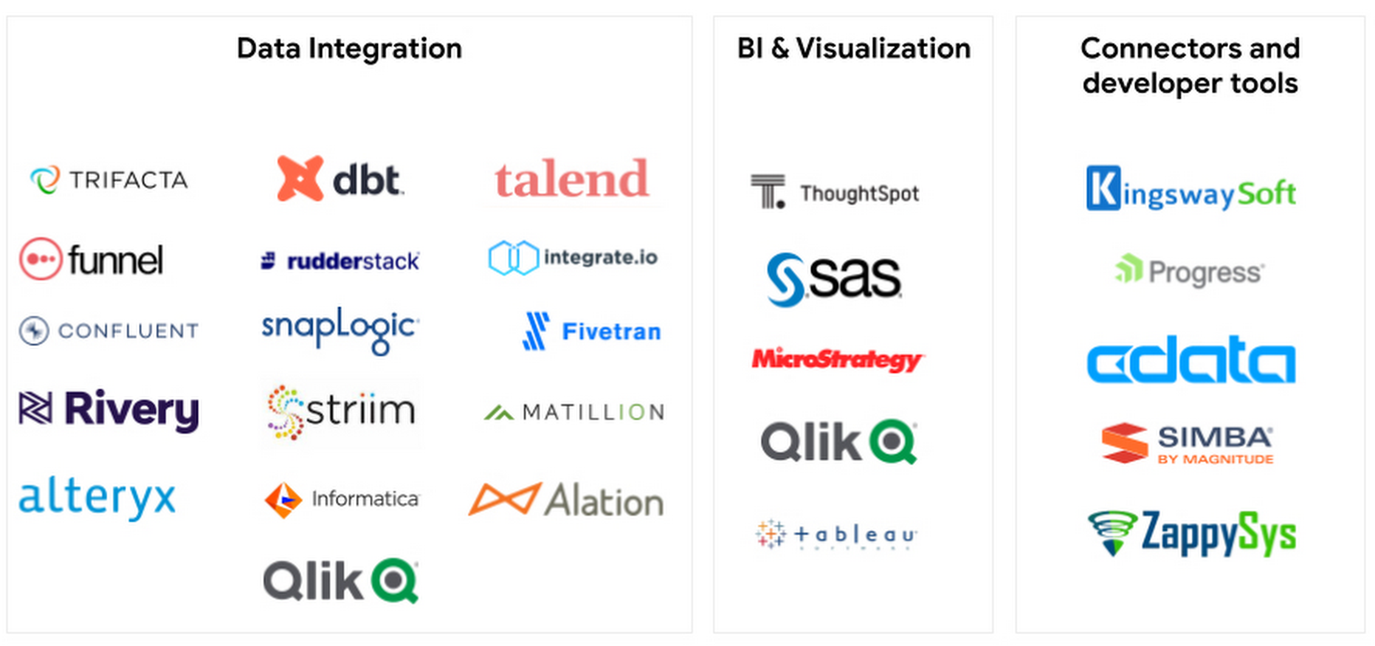
To enable this, we are launching a new Google Cloud Ready - BigQuery initiative. Google Cloud Ready - BigQuery is a validation program whereby Google Cloud engineering teams evaluate and validate BigQuery integrations and connectors using a series of data integration tests and benchmarks. Today, we’re announcing 25 launch partners whose integrations and connectors are validated as Google Cloud Ready - BigQuery:

For example, Google Cloud-validated connectors from Informatica help customers streamline data transformations and rapidly move data from any SaaS application, on-premises database, or big data source into Google BigQuery.

“Google Cloud and Informatica have been strategic cloud partners for the last five years, providing end-to-end, scalable enterprise-class data migration, integration and management solutions for customers. Being recognized as a Google Cloud Ready - BigQuery partner further validates Informatica's ability to help customers be successful in their journey to cloud with Google” said Jitesh Ghai, Chief Product Officer at Informatica.

Google Cloud-validated Fivetran connectors continuously replicate data from key applications, event streams, file stores, and more into BigQuery, helping turn big data into informed business decisions. Customers can keep up-to-date with the performance and health of the connectors through logs and metrics available through Google Cloud Monitoring. 

"Customers are looking to move data reliably and securely into Google BigQuery to meet the needs of their business," said Fraser Harris, VP of Product at Fivetran. "We are proud to announce that we have achieved Google Cloud Ready - BigQuery Designation. This marks another milestone in our long-standing partnership with Google Cloud that provides our customers with further assurance that Fivetran products work seamlessly with BigQuery - today and into the future."

Similarly, Google Cloud-validated BigQuery and Tableau integrations allow customers to analyze billions of rows in seconds without writing a single line of code and with zero server-side management. Organizations can create dashboards in minutes and share insights with users instantaneously.

“Tableau strives to meet customers where they are and for many organizations with large complex data problems, that’s on the Google Cloud Platform,” said Brian Matsubara, Vice President, Global Technology Alliances at Tableau. “Partnering with Google empowers our customers to explore their data in real-time to unlock actionable insights that can transform a business."

If you are already a Google Cloud partner, sign up to get your product integration validated by our experts. To become a Google Cloud partner, click here to enroll.

Helping ISVs build and grow their applications with BigQuery

More than 700 partners power their applications with Google’s data cloud - including companies like ZoomInfo, Equifax, Exabeam, Bloomreach, and Quantum Metric. We’re committed to helping these partners both build effective products and go to market, and this week we’re excited to launch the Built with BigQuery initiative, which helps ISVs get started building applications using data and machine learning products like BigQuery, Looker, Spanner, and VertexAI. The program provides dedicated access to Google Cloud expertise, training and co-marketing support to help partners build capacity and go to market. Furthermore, Google Cloud engineering teams work closely with our partners on product design and optimization, to share architecture patterns and best practices. This allows SaaS companies to harness the full potential of data to drive innovation at scale.

“Built with Google’s data cloud, Exabeam’s limitless-scale cybersecurity platform helps enterprises respond to security threats faster and more accurately” said Sanjay Chaudhary, VP of Products at Exabeam. “We are able to ingest data from over 500 security vendors, convert unstructured data into security events, and create a common platform to store them in a cost effective way. The scale and power of Google’s data cloud enables our customers to search multi-year data and detect threats in seconds”

Click here to learn more about the Built with BigQuery initiative.

Enhancing secure data sharing with Analytics Hub

We are also launching a public preview of Analytics Hub, a fully-managed service built on BigQuery that allows our data sharing partners to efficiently and securely exchange valuable data and analytics assets across any organizational boundary. With unique datasets that are always-synchronized, and bi-directional sharing, partners can create a rich and trusted data ecosystem

“As external data becomes more critical to organizations across industries, the need for a unified experience between data integration and analytics has never been more important. We are proud to be working with Google Cloud to power the launch of Analytics Hub, feeding hundreds of pre-engineered data pipelines from hundreds of external datasets,” said Dan Lynn, SVP Product at Crux. “The sharing capabilities that Analytics Hub delivers will significantly enhance the data mobility requirements of practitioners.”

Click here to join the public preview of Analytics Hub.

New launches from our data cloud partners

We’re excited to highlight several important launches from our partners themselves. At Google Cloud, we’re proud to support the fastest-growing and most innovative data and analytics companies, whether they’re running applications on Google Cloud, launching new integrations or connectors, co-creating entirely new capabilities with BigQuery, or continually tweaking and updating their platforms to provide the best experience for customers.

This week our partners Databricks, Fivetran, MongoDB, Neo4j, and Starburst Data are all announcing new capabilities for customers, including:

• Databricks SQL will be publicly available for all customers on Google Cloud this month, enabling customers to operate multi cloud lakehouse architectures with performant query execution. Learn more, here.

• Fivetran, in addition to joining the Cloud Ready - BigQuery initiative, is now a partner for the Google Cloud Cortex Framework. With deep experience in moving data from a variety of SaaS and database sources - including SAP, Fivetran offers Google Cloud customers accelerated time to value in unlocking the Google Cloud Cortex Framework data models, driving real-time analytics and business insights.

• MongoDB is working to launch real-time integration of operational data from Atlas to Google BigQuery (and vice versa) via Dataflow Templates. This enables customers to cross-reference operational data and leverage BigQuery and it’s Analytics, as well as AI/ML tools to support use cases such as anomaly detection in IoT, product recommendations in Retail and fault detection in Manufacturing and feed these insights back to MongoDB Atlas to power the modern real-time enabled enterprise for Continuous Intelligence. This is targeted to be available in Q3/22. 

• Neo4j is launching a fully-managed graph technology service for data scientists and developers to build intelligent, algorithm-powered applications with Neo4j Graph Data Science on Google Cloud.

• Starburst is announcing a packaged offer for customers to enrich their BigQuery data foundation with hybrid, cross-cloud data stores.

The depth and breadth of innovation and support from the Google Cloud ecosystem is a tremendous asset for customers as they accelerate their data-driven digital transformations. Our community of expert services partners and systems integrators are heavily engaged, too - to date, our partners have earned more than 80 Specializations and more than 200 Expertises pertaining to data cloud technologies on Google Cloud. Visit our partner directory to find partners specialized in Google’s data cloud.

If you are already a Google Cloud partner, sign up to get your product integration validated by our experts. If you are looking to build your applications on Google’s data cloud, apply for the Built with BigQuery initiative. To become a Google Cloud partner, click here to enroll.

Imagine your director sends you a chat message Monday morning: Our average order value dropped 7% in January, but total revenue stayed flat. Why?

If you’re a data practitioner, you know why these types of questions can be tough. They’re totally open ended. There’s not a single root cause dashboard you can open. Was there an error in the web logs? Was a promo code misconfigured? You won’t know until you start digging, and you rarely find the answer in just one place.

Each piece of the answer lives somewhere different in your environment:

• Sales history (orders and line items) sits in a data warehouse

• Live customer records are in a production PostgreSQL instance

• Marketing campaign rules are raw JSON files in an object store

Writing any one of these queries is easy. You’ll write the same one a dozen times, tweaking WHERE clauses or adding subqueries to find the answer. Then you’ll bounce to the next system and start again with a different dialect. Before you know it, you have ten browser tabs open and a whole afternoon gone, all to answer one question.

Data Agent Kit

The Data Agent Kit is built to solve this issue. It is a set of MCP servers and agent skills that helps data developers run data workflows from their IDEs. It’s available both as an extension for VS Code forks (Antigravity IDE, Cursor) and as a plugin for other tools (Antigravity 2.0, Antigravity CLI, Claude Code, Codex), so you don’t need to leave your IDE to get answers.

The Data Agent Kit relies on two core mechanisms:

• Model Context Protocol (MCP): an open standard that connects your agent to tools, databases, and remote cloud infrastructure.

• Skills: markdown files that augment your agent’s knowledge, teaching it how to interact with your specific stack.

Instead of generating SQL snippets and copy-pasting them into a console, Data Agent Kit lets agents run the queries and read the results on your behalf.

Let’s see what this looks like in practice applied to the average order value scenario. In this setup, the data warehouse is BigQuery, the Postgres instance is Cloud SQL, and the campaign rules sit in Cloud Storage.

Finding out what happened

The investigation begins in the IDE’s chat pane with the following natural language prompt to confirm the baseline numbers:

code_block

<ListValue: [StructValue([('code', 'Calculate our monthly average order value from August 2025 through January 2026 using the orders and order items tables in BigQuery.'), ('language', ''), ('caption', <wagtail.rich_text.RichText object at 0x7fc79cad5fd0>)])]>

Checking its work

The agent processes your prompt, invokes relevant skills, and prepares to start querying your data. But before it can execute anything, the IDE  pauses to ask for permissions to use the necessary MCP tools (e.g. execute_sql_readonly). You can allow it once for auditing, or select “always allow” to keep the workflow moving. Once approved, the agent sends off the queries.

Agentic IDEs allow you to inspect the execution trail, which reveals items like each MCP tool call or the raw SQL sent to BigQuery. It’s important to keep an eye on generated code, though reading a query can take much less time than writing one against schemas you’re unfamiliar with.

Breaking down the numbers

The numbers showed that average order value remained around $110 from August to December, but dropped to $103 in January. To find out why, ask the agent to drill down:

code_block

<ListValue: [StructValue([('code', "Break down January's AOV by order type to see what's going on"), ('language', ''), ('caption', <wagtail.rich_text.RichText object at 0x7fc79c8bd250>)])]>

The results point to a skewed average instead of a business decline. Online and Offline orders stayed healthy (~$110). A new channel called B2B-Wholesale appeared in January with an AOV of just ~$75. Nothing declined, but the product mix changed.

Crossing into Cloud SQL

You know what led to lower AOV. Next, you need to figure out who the wholesale buyers are. The customer records are stored in a Cloud SQL Postgres operational database, and you can continue in the same chat thread:

code_block

<ListValue: [StructValue([('code', 'Who are these B2B customers? Check our Cloud SQL database for their account details and creation dates.'), ('language', ''), ('caption', <wagtail.rich_text.RichText object at 0x7fc79c488c90>)])]>

The agent switches to the Cloud SQL MCP and inspects the customers table for you. All 100 wholesale accounts are brand-new business entities created within the last 30 days. None of them existed in December.

Dropping into the terminal

A quick glance at the B2B orders in BigQuery shows that 92% applied promo_code = BIGORDER25. You can then ask the agent to track that code back to the campaign files, and it will use the Google Cloud Storage MCP server to access the file.  

The marketing campaign shows a 25% discount code led to a huge number of low-priced wholesale orders, which reduced the blended AOV while total revenue remained flat.

In a single chat session, the agent queried analytical data (BigQuery), operational records (Cloud SQL), and unstructured metadata (Cloud Storage) to find the root cause.

Updating the director

Now, you can prompt the agent to return a short executive summary for your director.

And voilà! With a few natural language prompts straight from your IDE, you've answered the director's open ended question.

Root cause analysis is only part of the job. The next time this issue occurs, you won't want to run through the same situation. Instead, you can turn this investigation into a reproducible data model.

Build a reproducible pipeline

Ask the agent to turn your ad-hoc analysis into a persistent dbt project:

code_block

<ListValue: [StructValue([('code', 'Build a dbt project that joins our BigQuery staging models with our Cloud SQL customer and pet profile attributes. Add a uniqueness test on order_id and run dbt build.'), ('language', ''), ('caption', <wagtail.rich_text.RichText object at 0x7fc79c48a0d0>)])]>

From a single prompt, the agent creates a virtual Python environment with dbt-bigquery and writes project models and tests. But then dbt build fails. The uniqueness test catches duplicates on order_id.

Customers can own more than one pet. The first version of the model attached those profiles directly to each order, so an order from a three-pet household became three rows (not unique).

The agent reads its own terminal output and catches the failure. It then rewrites the dbt logic and reruns it until the build passes.

This introduces an important note about agentic workflows. Agents are capable of writing mountains of code - but you'll still need to apply data quality checks to your pipeline (fortunately, an agent can write those too).

The next time leadership asks why average order value moved, you'll have a dbt model ready to answer it.

Wrap up

An agentic IDE keeps you from bouncing between your warehouse, your databases, your object store, and your terminal.

By pairing open standards like MCP and modular (and editable!) agent skills, the Data Agent Kit removes the friction between question and answer. Combing through unfamiliar schemas, translating between dialects, writing the joins you’ve written a hundred times: that becomes the agent’s job. You’re in charge of directing the investigation.

Try it yourself

The Data Agent Kit is in preview and works natively in Antigravity (2.0, CLI, IDE), Claude Code, Codex, Cursor, and other popular tools.

• Try the Scenario: walk through the full setup in the Analytics with Data Agent Kit and Antigravity IDE Codelab.

• Read the Docs: learn more at the Google Cloud Data Agent extension documentation.

• Explore the Plugin: check out the skills and tools in the open-source repository on GitHub.

As a global media and technology company connecting hundreds of millions of users to finance, sports, and entertainment platforms, Yahoo operates a massive data infrastructure where analytics workloads must run continuously at high speed. In deadline-driven data environments, relying on fixed virtual machine (VM) configurations creates a brittle system; if a specific machine shape faces a regional capacity constraint, cluster provisioning in Managed Service for Apache Spark (formerly Dataproc) can experience delays and stall critical data pipelines.

Yahoo utilizes flexible VMs in Managed Service for Apache Spark clusters to automatically absorb these resource fluctuations by defining a ranked list of acceptable VM shapes. This allows the system to dynamically search regional zones and maintain pipeline execution without manual intervention. To search for capacity across a region, teams must also enable Auto-Zone placement.

This optimization builds on Yahoo's broader data modernization journey, which involved migrating on-premises Hadoop and big data estates directly to Google Cloud. By transitioning those legacy workloads, the team established a cloud foundation capable of running high-scale batch and streaming analytics with dynamic resource flexibility.

This post provides a technical blueprint for configuring flexible VM instance rankings in Managed Service for Apache Spark to automatically manage capacity constraints and maintain pipeline execution.

Operational trade-offs of static configurations

Configuring clusters with a single, fixed machine type in a specific zone introduces constraints when regional zonal capacity fluctuations occur, potentially impacting cluster provisioning. Rather than manage these capacity variations through custom retry logic or manual intervention, using flexible configurations allows your infrastructure to automatically adapt. By accepting multiple VM shapes and searching across zones in the selected region, flexible configurations help streamline provisioning to better support high-scale analytics workloads.

Rules for configuring flexible clusters

Deploying flexible configurations requires aligning several connected design choices:

• Enable auto-zone placement: You must pass a region(--region=${REGION}) or an empty zone string (--zone="") so Managed Spark can search for available capacity across the entire region.

• Maintain core and memory symmetry: If your Managed Spark cluster uses autoscaling, all machine types in your flexible list must share a similar core count and memory size, even if they come from different VM families. A uniform CPU-to-memory ratio across primary and secondary workers prevents performance degradation, as the smallest ratio determines your effective container sizing.

• Align component properties: Managed Spark calculates system properties based on VM cores and memory. When mixing machine shapes, you may need explicit property overrides to keep YARN and Spark resource allocations aligned with your expected worker behavior.

Two ways flexible VMs support massive workloads

For large-scale data environments, flexible configurations support operations in two ways:

1. Higher cluster creation success: Instead of failing when a preferred VM type is out of stock, Managed Spark selects from a ranked list to keep provisioning moving.

2. Better regional resource use: Auto-zone placement searches the entire region to find capacity, which reduces provisioning friction during high-demand periods.

gcloud example

code_block

<ListValue: [StructValue([('code', 'gcloud dataproc clusters create analytics-cluster \\\r\n --region=us-central1 \\\r\n --zone="" \\\r\n --num-workers=10 \\\r\n --master-instance-selection=\'{"machineTypes":["e2-standard-8"],"rank":0}\' \\\r\n --master-instance-selection=\'{"machineTypes":["n2-standard-8"],"rank":1}\' \\\r\n --worker-instance-selection=\'{"machineTypes":["e2-standard-8"],"rank":0}\' \\\r\n --worker-instance-selection=\'{"machineTypes":["n2-standard-8"],"rank":1}'), ('language', ''), ('caption', <wagtail.rich_text.RichText object at 0x7f8e31ac9450>)])]>

API example

You can also build this capacity policy into your automated pipelines or Managed Service for Apache Airflow DAGS using the instanceFlexibilityPolicy field in the ‘Dataproc’ API:

code_block

<ListValue: [StructValue([('code', '{\r\n "projectId": "PROJECT_ID",\r\n "clusterName": "analytics-cluster",\r\n "config": {\r\n "gceClusterConfig": {\r\n "zoneUri": ""\r\n },\r\n "secondaryWorkerConfig": {\r\n "numInstances": 8,\r\n "instanceFlexibilityPolicy": {\r\n "instanceSelectionList": [\r\n {\r\n "machineTypes": ["n2-standard-8"],\r\n "rank": 0\r\n },\r\n {\r\n "machineTypes": ["e2-standard-8", "t2d-standard-8"],\r\n "rank": 1\r\n }\r\n ]\r\n }\r\n }\r\n }\r\n}'), ('language', ''), ('caption', <wagtail.rich_text.RichText object at 0x7f8e32253250>)])]>

This API policy achieves the same goal: it establishes your preferred shape, documents valid fallbacks, and lets Managed Spark resolve resource constraints without breaking your automation scripts.

Establishing an infrastructure policy

Managing data at this scale requires standardizing a clear resource policy rather than relying on a single rigid machine type. Your configuration standards should outline:

• Preferred and fallback VM families for secondary workers.

• Default auto-zone placement to enable flexible provisioning.

• Identical core and memory configurations when using autoscaling.

• Uniform CPU-to-memory ratios across all worker groups to maintain predictable container sizing.

• Explicit YARN or Spark property overrides to guarantee consistent runtime behavior across different machine lines.

• Shuffle-safe patterns for Spark workloads running on Spot or highly elastic capacity.

By adopting flexible configurations, you turn infrastructure scarcity into a predictable fallback plan, keeping your critical data pipelines up and running.

Yahoo impact and results

By implementing flexible VMs in Managed Service for Apache Spark, Yahoo successfully reduced cluster provisioning failures by 85% which were caused by regional capacity stockouts. This flexible configuration allows their data infrastructure to automatically handle capacity constraints and successfully provision resources without requiring manual intervention. As a result, Yahoo ensures continuous workload execution and prevents downstream processing delays across their massive data pipelines.

"Managing high-scale data analytics at Yahoo requires resilient, automated infrastructure. Moving to flexible VMs in Managed Service for Apache Spark has transformed our approach; instead of stalling when a specific machine shape faces capacity constraints, our clusters now automatically pivot to our ranked fallback options. This has helped us reduce provisioning failures by 85%, providing the reliability we need to keep our global media platforms running smoothly." - Akshay Jain, Senior Software Developer Engineer, Yahoo!

Strategic benefits of flexible infrastructure

Adopting a flexible compute stack transforms your environment into a dynamic pool of resources that adapts to your operational needs. By moving away from rigid, single-machine type configurations, you ensure that your workloads reliably access the compute they need, regardless of supply fluctuations. This shift not only maximizes workload obtainability and reliability but also facilitates seamless hardware modernization by allowing you to prioritize newer VM generations while maintaining older types as reliable fallback options.

Build your resilient data pipeline

Transitioning to a fluid compute strategy ensures your critical analytics remain operational despite regional resource shifts. Here is how you can begin optimizing your infrastructure today:

1. Audit your workloads: Identify applications tightly coupled to specific VM families or zones and map out viable alternative hardware shapes.

2. Standardize resource policies: Explore the documentation for Managed Spark flexible VMs to establish your preferred and fallback VM families.

3. Align financial strategy: Utilize Flexible Committed Use Discounts (Flex CUDs) to maintain cost predictability when workloads dynamically pivot to alternative machine types.

4. Claim your credits: New customers may be eligible for $300 in credits to try Managed Service for Apache Spark and other Google Cloud products at no cost.

September 7 - September 10

• Pub/Sub SMTs can now AI Inference your Gemini Enterprise Agent Platform models!
  Pub/Sub AI Inference SMTs allow you to apply inference on an incoming stream of events using models hosted in Gemini Enterprise Agent Platform. The model’s prediction is appended to your event, making it available for downstream processing in your data warehouse (like BigQuery) or operational database (like BigTable). This feature, now generally available, can dramatically simplify or enhance anomaly detection systems you are operating. 

• PostgreSQL Source Connector is now generally available in Managed Service for Apache Kafka!
  Managed Service for Apache Kafka’s PostgreSQL connector allows customers to capture changes from their PostgreSQL database and ingest them into their Kafka infrastructure with low latency. This source connector is compatible with Cloud SQL for Postgres, AlloyDB, and self-managed PostgreSQL databases. Try this along with our entire portfolio of managed connectors, including MirrorMaker 2.0, BigQuery, Cloud Storage, and Pub/Sub! E-mail kafka-hotline@google.com if you have questions or feedback!

• Pause-on-failure for Dataflow batch jobs is GA
  Dataflow pause-on-failure enables you to preserve the state of a batch Dataflow job before it fails. By pausing your Dataflow job, you can address issues that are external to the pipeline and resume processing without losing completed work. This helps you better manage resource costs and improve job reliability when you face temporary outages or capacity constraints.

• The insertAll API is now the BigQuery Storage Write API (REST)
  The legacy insertAll streaming API is now rebranded as the BigQuery Storage Write API (REST). By dropping the "legacy" label, developers can confidently build long-term HTTP-based streaming workflows. This stateless JSON-over-HTTPS endpoint offers a lightweight alternative to heavy gRPC libraries—ideal for serverless web apps, IoT telemetry, and AI logging. The transition is seamless for existing users, requiring zero code changes and offering 100% backward compatibility. However, the Storage Write API (gRPC) version remains the recommended standard for high-throughput, continuous pipelines.

August 31 - September 4

• Stateful processing is available in BigQuery continuous queries in Preview
  Stateful operations significantly expand what’s possible with BigQuery continuous queries. This feature allows users to leverage functions like JOINs, aggregations, and windowing functions directly in their streaming queries. Now you can calculate metrics over time (for example, a 30-minute average) to power your downstream applications and AI agents with much richer, real-time signals.
  
  Try out our feature here and share your feedback with bq-continuous-queries-feedback@google.com!

• Synthetic data generator tool is available for Managed Service for Kafka
  You’ve launched your first Kafka cluster. Now what? The next thing to do is to produce some data to the cluster, but that involves modifying a client application somewhere or spinning up a virtual machine. The synthetic data generator tool, now generally available, can start sending mock data to your cluster in 3 clicks, and will get data streaming into your cluster in less than two minutes. The perfect utility for those moments you just want to test your cluster and new features. Try our quickstart today!

• Dataflow pipeline updates are faster & more flexible
  Dataflow pipeline updates can now stop-and-replace pipelines, a major addition to the existing in-place-update feature. The new parallel pipeline option accelerates the migration between the old & new pipeline, resulting in reduced disruption to your business. You can also set a timeout on drains that prevents runaway costs for your pipeliness in the event of stuck processing. This feature is generally available. Try it here!

July 6 - July 10

• New Lakehouse managed tables now in preview
  Lakehouse tables for Apache Iceberg are now in preview and available in the console. By using Google-managed Apache Iceberg tables in Lakehouse, you can eliminate the overhead of maintaining duplicate data pipelines and complex synchronization logic between BigQuery and open-source engines. This unified table format delivers native, multi-engine read and write interoperability, allowing you to run concurrent DML/DDL operations across diverse analytics tools on a single, shared storage layer.  Built-in automated table management handles painful background optimization tasks like compaction and partition tuning, freeing up your team to focus on building rather than managing storage maintenance.

June 1 - June 5

• Beyond the Query: Powering AI Agents with Bigtable, Firestore & Memorystore
  Discover the latest advancements in Google Cloud's NoSQL Database portfolio, including Bigtable, Firestore, and Memorystore. This series is designed for a broad audience: whether you are exploring these databases for the first time or are an existing user looking to leverage the new capabilities announced at Next '26.
  
  Register here to secure your spot!

• Cloud Engineer's AI Toolkit Workshops: Solve data-driven challenges with BigQuery, AlloyDB, Gemini and more. Hosted by Google Cloud Labs, this highly technical event is built specifically for Platform Engineers, SREs, and cloud infrastructure teams ready to bridge the gap between AI prototypes and production-grade deployments. Look out for more locations coming soon
  
  Toronto - June 25 (Data Cloud) | RSVP Here
  Chicago - June 30 (Data Cloud) | RSVP Here

• Start a 10-day Bigtable free trial with a 1 node SSD cluster and up to 500GB of storage capacity. With no credit card required to start, you can easily ingest workloads and manage workloads that require low-latency, high-throughput, and predictable access. Plus, new Google Cloud customers get $300 in free credits on signup.

May 11 - May 15

• Managed Service for Apache Airflow has launched a wave of new features, including the general availability of Airflow 3.1, AI-powered agentic troubleshooting, a new managed Airflow MCP Server for custom agent integration, and declarative YAML-based orchestration pipelines—discover all the details in the full blog post.

April 20 - April 24

• Google-built ODBC Driver for BigQuery is now available in Preview
  We are excited to announce the launch of the new, Google-built ODBC driver for BigQuery. This new open-source driver provides a direct, high-performance connection for applications to BigQuery and is developed entirely in-house by Google. Download a new driver and connect your application to BigQuery.

April 13 - April 17

• We announced we are reintroducing Data Studio to play a significant role in the AI era, expanding from data visualizations and reports to host BigQuery conversational agents and data apps built in Colab notebooks.
• We announced BigQuery Graph is now available in preview, offering an easy-to-use, highly scalable graph analytics solution, empowering data professionals to model, analyze and visualize massive-scale relationships in an entirely new way.

April 6 - April 10

• We introduced Conversational Analytics for Looker Embedded environments, enabling users to add natural language experiences to their own custom data-driven applications, powered by Gemini. 
• We expanded Looker’s capabilities for faster ad-hoc analysis, with the introduction of self-service Explores, enabling you to bring your own data to Looker’s semantic layer and gain instant access to insights in a governed data environment.

March 23 - March 27

• We showed you how you can scale your reads with Cloud SQL autoscaling read pools. This feature allows you to provision multiple read replicas that are accessible via a single read endpoint and to dynamically adjust your read capability based on real-time application needs. 
• Our customers are leveraging the full power of Conversational Analytics and Looker to drive major business and technical breakthroughs in the AI era. Companies like Telenor, Pet Circle, Fluent Commerce, Lighthouse Intelligence, Wego, and ROLLER are turning data into insights and actions, grounded by Looker’s semantic layer.

March 16 - March 20

• We introduced an enhanced Gemini assistant in BigQuery Studio, transforming the agent from a code assistant into a fully context-aware analytics partner.

February 23 - February 27

• We introduced managed and remote MCP support for Google Cloud databases, including AlloyDB, Spanner, Cloud SQL, Bigtable and Firestore, to power the next generation of agents. This announcement extends the ability for AI models to plan, build, and solve complex problems, connecting to the database tools our customers leverage daily as the backbone of their work environment.

• We outlined how you can build a conversational agent in BigQuery using the Conversational Analytics API to help you build context-aware agents that can understand natural language, query your BigQuery data, and deliver answers in text, tables, and visual charts.

February 16 - February 20

• Our customers are leveraging the full power of Looker to drive major business and technical breakthroughs. Companies like Arrive, Audika, Carousell, Framebridge, GumGum, Intel, Overdose Digital, Ocean Network Express, Subskribe and Promevo are leveraging Looker’s newest AI-driven capabilities, including Conversational Analytics, to transform data to insights and actions, and empower their entire organization with a single source of truth, powered by Looker’s semantic layer.

February 2 - February 6

• Join us on March 4 for our webinar, Win Your AI Strategy with Cloud SQL Enterprise Plus, to learn how to power your generative AI workloads with 3x higher performance and 99.99% availability. Register today to discover how to build a scalable, enterprise-grade foundation for your most demanding AI applications.

January 26 - January 30

• We introduced Conversational Analytics in BigQuery, which allows users to analyze data using natural language. Conversational Analytics in BigQuery is an intelligent agent that generates, executes and visualizes answers grounded in your business context directly in BigQuery Studio, making data insights for data professionals more conversational.
• We outlined how data products have become the foundation for AI agents, providing the context needed to make autonomous agents reliable and trusted for real business use, backed by organized business logic and semantic understanding.
• We highlighted how you can supercharge data analytics workflows, and outlined Google Cloud’s AI agent offerings for data engineering, data science, and development tools, so you can integrate agentic workflows in your applications, empower your teams and speed discovery.

January 19 - January 23

• We have fundamentally reimagined Firestore with pipeline operations for Enterprise edition. Experience a powerful new engine featuring over a hundred new query features, index-less queries, new index types, and observability tooling to improve query performance. Seamlessly migrate using built-in tools and leverage Firestore’s existing differentiated serverless foundation, virtually unlimited scale, and industry-leading SLA. Join a community of 600K developers to craft expressive applications that maximize the benefits of rich queryability, real-time listen queries, robust offline caching, and cutting-edge AI-assistive coding integrations.

• Introducing Google Cloud SQL on MSSQLTips: We are highlighting a new technical guide published on MSSQLTips titled "Introducing Google Cloud SQL." This article serves as an essential resource for SQL Server administrators and developers exploring Google Cloud's fully managed database service. It provides a detailed overview of Cloud SQL capabilities, including high availability, security integration, and the seamless transition of on-premises SQL Server workloads to the cloud, making it an ideal resource for those planning their migration strategy.

• We are excited to announce the Public Preview of Microsoft Entra ID (formerly Azure Active Directory) integration with Cloud SQL for SQL Server. Designed to tackle the challenge of identity sprawl in multi-cloud environments, this integration allows organizations to govern database access using their existing Microsoft identity infrastructure. Key benefits include centralized identity management, enhanced security features like Multi-Factor Authentication (MFA), and simplified user administration through direct group mapping. This feature is available for SQL Server 2022 and supports both public and private IP configurations.

January 12 - January 16

• Google-built JDBC Driver for BigQuery is now available in Preview
  We are excited to announce the launch of the new, Google-built JDBC driver for BigQuery. This new open-source driver provides a direct, high-performance connection for Java applications to BigQuery and is developed entirely in-house by Google. Download a new driver and connect your Java application to BigQuery.
• Troubleshoot Airflow tasks instantly with Gemini Cloud Assist investigations: Cloud Composer just got smarter. We are excited to announce that Gemini Cloud Assist investigations are now available directly within Cloud Composer 3. Instead of manually sifting through raw logs, you can now simply click "Investigate" on a failed Airflow task. Gemini analyzes logs and task metadata to identify failure patterns—such as resource exhaustion or timeouts—and provides actionable recommendations driven by Gemini Cloud Assist to resolve the issue. This integration shifts the debugging experience from manual toil to automated root cause analysis, significantly reducing the time required to restore your pipelines. Learn more about AI-assisted troubleshooting.

To further empower our customers in their data journey, we are excited to announce the launch of identity columns in BigQuery. This new feature allows users to define columns that automatically generate sequential 64-bit integer values, simplifying the way you manage unique identifiers within your tables.

Data engineers are always looking for ways to make data ingestion smoother and more reliable. BigQuery identity columns offer a powerful, built-in mechanism to automatically generate unique numerical values for your tables. By shifting the responsibility of ID generation to BigQuery, you can significantly reduce the complexity of your data pipelines and focus on delivering insights.

Key benefits for your data pipelines

Implementing identity columns provides several advantages that help streamline the development and maintenance of your data architecture.

• Streamlined ingestion: You can now ingest data without needing to pre-calculate unique keys in your application logic or ETL tools.

• Reduced boilerplate: By using auto-generated sequences, your SQL code becomes cleaner and easier to maintain, as the database handles key management natively.

• Integrated automation: Identity columns work harmoniously with standard DML operations, ensuring that every new row receives a unique identifier automatically.

• Flexible integration: Whether you are using INSERT or MERGE statements, identity columns adapt to your existing workflow.

How to implement identity columns

Setting up an identity column is simple and can be done directly within your CREATE TABLE statement. You have two primary ways to define how these values are handled.

Definition options

Example usage
The following SQL statement demonstrates how to create a table that automatically increments IDs, starting at 1 and increasing by one for each new entry.

code_block

<ListValue: [StructValue([('code', "CREATE TABLE my_project.my_dataset.orders (\r\n order_id INT64 GENERATED ALWAYS AS IDENTITY (START WITH 1 INCREMENT BY 1),\r\n customer_name STRING,\r\n order_date DATE\r\n);\r\n\r\n-- Ingesting data is now simpler:\r\nINSERT INTO my_project.my_dataset.orders (customer_name, order_date)\r\nVALUES ('Joe Doe', CURRENT_DATE());"), ('language', ''), ('caption', <wagtail.rich_text.RichText object at 0x7fcc84da5c50>)])]>

Get started today

Identity columns represent our ongoing commitment to providing a flexible, high-performance, and standards-compliant data platform. By automating the generation of surrogate keys, we are making it easier for you to build scalable and maintainable data architecture.

To learn more about how to implement this feature in your projects, please visit the BigQuery identity columns documentation.

Historically, enterprise predictive analytics tasks such as predicting churn, purchase intent, or fraud scoring have meant building custom models using libraries like XGBoost, Random Forest, or Deep Neural Networks (DNNs). While effective, the traditional train-tune-deploy-retrain cycle can be complex and time-consuming. Additionally, the overhead of manual feature engineering, hyperparameter tuning, lengthy and expensive training, and the need for specialized data science skills can lead businesses to underutilize predictive models in their decision-making. 

Today, we are announcing the TabFM model in BigQuery. Developed by Google Research, TabFM is a state-of-the-art, pre-trained foundation model for regression and classification on tabular data. It leverages in-context learning (ICL) to deliver highly accurate predictions on your tabular datasets instantly via a single SQL statement, removing the separate training and deployment steps. TabFM on BigQuery is currently in preview. 

Here is what TabFM brings to your BigQuery analytics:

• Zero-shot predictions: Skip model training, tuning, and artifact deployment. Simply pass your labeled historical data and new prediction tables into a single SQL function to get instant, high-quality predictions.
• Predictive ML for your agentic applications: Building an agent for your business use? Add predictive powers to it with TabFM plus BigQuery MCP server. No runtimes or infrastructure to manage, just data in and predictions out.
• State-of-the-art accuracy: Outperforms custom-trained, out-of-the-box traditional models on complex datasets, achieving superior accuracy scores on industry benchmarks.
• Simple developer experience: Runs natively in BigQuery and is accessible via simple SQL syntax. Automatically handles featurization tasks such as missing values, categorical encoding, etc., with no complex feature engineering pipelines to manage.
• Scalability: Processes massive inference tables (up to millions of rows) in minutes using BigQuery’s distributed inference architecture.

The leading model for tabular predictions

Google’s TabFM delivers industry-leading accuracy across a wide range of tabular data. In evaluations on the TabArena benchmark, TabFM consistently outperforms both classic machine learning models and other tabular foundation models.

Learn more about the TabFM model here.

Getting started with TabFM in BigQuery

Using TabFM is straightforward. It is exposed directly through new, built-in SQL functions: AI.PREDICT and AI.EVALUATE.

1. Get instant predictions with AI.PREDICT
To make predictions, you write a single query that passes your training  data and prediction data. The model automatically infers whether the task is a classification or regression problem based on the data type of your target label.

code_block

<ListValue: [StructValue([('code', "-- Classifying transactions as fraudulent or not\r\nSELECT *\r\nFROM AI.PREDICT(\r\n TABLE `my_project.my_dataset.historical_transactions`, -- Training data (in-context examples)\r\n TABLE `my_project.my_dataset.new_transactions`, -- Prediction data\r\n label_col => 'is_fraud'-- Target column to predict\r\n);"), ('language', ''), ('caption', <wagtail.rich_text.RichText object at 0x7fa6f05bb210>)])]>

In this example, the output contains all original columns from your prediction table plus predicted label and probability columns (e.g. predicted_is_fraud). No manual feature engineering or model creation was required.

2. Evaluate models with AI.EVALUATE
You can quickly check prediction performance against a test set using the AI.EVALUATE function. This allows you to generate standard evaluation metrics in a single step.

code_block

<ListValue: [StructValue([('code', "-- Regression Evaluation for Customer Lifetime Value (LTV)\r\nSELECT *\r\nFROM AI.EVALUATE(\r\n TABLE `my_project.my_dataset.historical_customer_ltv`,\r\n TABLE `my_project.my_dataset.test_customer_ltv`,\r\n label_col => 'ltv'\r\n);"), ('language', ''), ('caption', <wagtail.rich_text.RichText object at 0x7fa6f24557d0>)])]>

AI.EVALUATE returns a robust set of metrics such as r2_score, mean_absolute_error etc. for regression problems and metrics such as precision, recall, and f1 for classification problems.

TabFM in BigQuery under the hood

Traditional machine learning requires fitting model parameters to a training dataset. TabFM, in contrast, uses in-context learning. Similar to how large language models (LLMs) learn a task from few-shot examples in a prompt, TabFM reads your training table as in-context examples and generates predictions for your target table in a single forward pass.

To handle the computational complexity and memory footprint of tabular foundation models, BigQuery performs distributed, parallelized inference on your data. Further, to optimize performance and resource utilization, it uses intelligent training-data sampling as well as distributed execution. This allows BigQuery to handle large input rows for training data while executing predictions quickly and efficiently across millions of rows of inference data.

Choosing the right tool for the job

TabFM introduces groundbreaking zero-shot capabilities to BigQuery, and complements existing offerings such as XGBoost models. Here’s how to choose between TabFM and other models:

• Use TabFM when you need rapid, high-quality predictive insights without machine learning expertise, when historical datasets are small-to-medium sized, when data changes frequently, and when you need to retrain your models frequently to maintain accuracy. It is also a great fit for conversational or agentic workflows where you need predictive analysis on demand.

• Use traditional models like XGBoost when you have very large historical datasets, require complete control over custom hyperparameter tuning, have a high number of features that exceed current limits of TabFM, or need feature-importance explainability, i.e., which of the input features contributed most to the prediction.

Predictive machine learning made easy

With TabFM natively integrated into BigQuery, predictive ML is now as easy as running a standard SELECT query. By eliminating the manual overhead of model training, tuning, and management, TabFM lets developers, data scientists and analysts go from raw data to rich predictive insights in seconds.

To get started today, check out the public documentation. For questions or feedback reach out to our team at bqml_feedback@google.com.  We look forward to seeing what you build!

Data pipelines are the backbone of the modern enterprise, yet a barrier to entry exists for orchestrating them, making this critical capability unavailable to many data professionals. Following our announcements at Google Cloud NEXT ’26, where we introduced the Orchestration Pipelines framework, we are fundamentally changing this dynamic.

To bring this powerful framework directly to practitioners, we offer the Data Agent Kit — a unified, freely available, and open-source collection of data engineering and data science tools that integrate directly into your preferred IDE or CLI (such as VS Code, Claude Code, or Codex).

The Data Agent Kit seamlessly embeds the Orchestration Pipelines framework into your workflow in two distinct ways. First, it provides a dedicated Data Engineering tab for comprehensive pipeline management. Second, it includes a specialized agentic skill designed to author, deploy, and troubleshoot production-grade Apache Airflow® DAGs using natural language.

By pairing these specialized agent skills with a declarative YAML DSL, all data personas — from analysts to ML engineers — can bypass complex Python Airflow boilerplate. This framework decouples high-level orchestration logic from underlying compute execution, democratizing access to powerful MLOps capabilities across your entire data organization.

In this post, we will walk through an exemplary MLOps use case to demonstrate how easily this can be achieved.

Setting up your environment

Before authoring your first Orchestration Pipeline, you need to set up your local development environment. Getting started takes less than two minutes.

1. Install and configure the extension

To install the extension in your preferred IDE or CLI — such as VS Code, VS Code forks, Antigravity, Claude Code, Antigravity CLI, or Codex — and authenticate it with your Google Cloud account, follow the step-by-step setup guide in the official documentation: Google Cloud Data Agent Kit installation guide

2. Verify orchestration pipeline skills

Once installed, verify that the required agent skills are active:

1. Open the ‘Google Cloud Data Agent Kit’ panel on the VS Code activity bar.

2. Navigate to ‘Settings’ then ‘Skills’.

3. Ensure the ‘gcp-pipelines-orchestration’ skill is enabled.

This skill provides the agent with deep contextual knowledge of pipeline syntax, variable substitution, secret management, and automated incident diagnosis for Airflow runs.

3. Building your first pipeline

To start authoring, building, and validating orchestration pipelines directly inside the any VS Code compatible IDE using natural language prompts, follow the official building guide: Build pipelines guide

An example business problem: Proactive supply chain management

Let’s walk through an example business problem. In the logistics and retail sector, customer satisfaction hinges on accurate delivery estimates. When an order is delayed without warning, customer churn can spike and support costs can escalate.

To address this, we are building an end-to-end MLOps architecture that predicts the exact transit time (in days) based on warehouse location, customer location, and order characteristics. By predicting these delays before shipping, operations teams can proactively notify customers or automatically upgrade shipping tiers before Service Level Agreements (SLAs) are breached.

To make this architecture fully reproducible, we use the bigquery-public-data.thelook_ecommerce public dataset in BigQuery. For demo purposes, we split this static dataset into training and inference sets. In a real-life scenario, inference would be performed on new, incoming data. This dataset provides authentic operational complexity:

• Geographical data: Latitude and longitude for both customer addresses (users) and distribution centers (distribution_centers).

• Temporal data: Granular order lifecycle timestamps (created_at, shipped_at, delivered_at).

• Order attributes: Product categories, pricing, and fulfillment status (orders, order_items).

By combining this dataset with BigQuery, Managed Service for Apache Spark serverless, Gemini Enterprise Agent Platform, and dbt, we will demonstrate how to build an automated, self-healing MLOps loop that handles training, daily batch inference, and model drift evaluation.

The agentic workflow: From prompt to pipeline in minutes

With the extension configured, we can bypass boilerplate Python for DAG authoring entirely. Inside VS Code, we opened the Data Agent Kit chat and provided a single natural language prompt to define our continuous MLOps feedback loop:

Note: The detailed prompt was crafted with repeatability in mind specifically for this blog post. In real-life scenarios, you can achieve the same result in a more conversational way, pipeline by pipeline. The complete prompt and all generated files are available in the Orchestration-pipelines GitHub repository. 

Note: While frontier models equipped with the Orchestration Pipelines skill can often scaffold complete workflows in a single step, LLM responses naturally vary based on model versions, workspace context, and token depth. If a specific parameter, dataset path, or dependency is omitted in the initial pass, simply provide a short follow-up prompt.

Within minutes, the Data Agent Kit generated the underlying PySpark scripts, dbt configurations, and the three declarative YAML pipelines.

Please find below the generated YAML pipelines and a visual diagram of them. This pipeline is a simplified example designed to showcase Orchestration Pipelines capabilities. In practice, recommended production MLOps setups will vary depending on your specific use cases and operational needs.

Pipeline 1: The training engine
This pipeline serves as our heavy-compute engine. The agent generated a YAML definition that first queries BigQuery to extract historical completed orders. It then dynamically provisions a Managed Spark serverless cluster to calculate geographical distances and train a model for production use. Finally, it pushes the trained model to Gemini Enterprise Agent Platform Model Registry.

code_block

<ListValue: [StructValue([('code', 'modelVersion: "1.0"\r\npipelineId: "training-pipeline"\r\nrunner: airflow\r\nowner: "mlops"\r\ntags:\r\n - "job:datacloud:antigravity"\r\ndefaults:\r\n projectId: "your-project-id"\r\n location: "us-central1"\r\n executionConfig:\r\n retries: 0\r\n\r\nactions:\r\n - sql:\r\n name: "extract_training_data"\r\n engine:\r\n bigquery:\r\n location: "US"\r\n destinationTable: "your-project-id.mlops.training_dataset"\r\n query:\r\n path: "blogpostdemo/training_query.sql"\r\n\r\n - pyspark:\r\n name: "train_model_dataproc"\r\n dependsOn:\r\n - "extract_training_data"\r\n engine:\r\n dataprocServerless:\r\n location: "us-central1"\r\n resourceProfile:\r\n inline:\r\n runtimeConfig:\r\n version: "2.3"\r\n properties:\r\n "spark.dataproc.driverEnv.PYTHONPATH": "./libs/lib/python3.11/site-packages"\r\n "spark.executorEnv.PYTHONPATH": "./libs/lib/python3.11/site-packages"\r\n mainFilePath: "blogpostdemo/train_model.py"\r\n environment:\r\n requirements:\r\n inline:\r\n list:\r\n - "tensorflow==2.14.1"\r\n - "numpy<2.0.0"\r\n - "protobuf<5.0.0dev"\r\n - "google-cloud-storage"\r\n\r\n - ai:\r\n name: "upload_model_vertex"\r\n dependsOn:\r\n - "train_model_dataproc"\r\n agentPlatform:\r\n projectId: "your-project-id"\r\n location: "us-central1"\r\n modelUpload:\r\n modelName: "transit_days_predictor"\r\n modelArtifactUri: "gs://your-bucket-name/models/tf_transit_days_model"\r\n servingContainerImageUri: "us-docker.pkg.dev/vertex-ai/prediction/tf2-cpu.2-14:latest"'), ('language', ''), ('caption', <wagtail.rich_text.RichText object at 0x7febd5a366a0>)])]>

Pipeline 2: Daily inference
For our daily operational workflow, this lightweight pipeline applies the trained model to all currently in-transit orders. It queries the dataset via BigQuery job, executes inference job via Gemini Enterprise Agent Platform, and writes the results back to a BigQuery table to flag potential SLA breaches for the customer support team.

code_block

<ListValue: [StructValue([('code', 'modelVersion: "1.0"\r\npipelineId: "inference-pipeline"\r\nrunner: airflow\r\nowner: "mlops"\r\ntags:\r\n - "job:datacloud:antigravity"\r\ndefaults:\r\n projectId: "your-project-id"\r\n location: "us-central1"\r\n executionConfig:\r\n retries: 0\r\n\r\nactions:\r\n - sql:\r\n name: "extract_inference_data"\r\n engine:\r\n bigquery:\r\n location: "US"\r\n destinationTable: "your-project-id.mlops.inference_dataset"\r\n query:\r\n path: "blogpostdemo/inference_query.sql"\r\n\r\n - ai:\r\n name: "run_vertex_batch_prediction"\r\n dependsOn:\r\n - "extract_inference_data"\r\n agentPlatform:\r\n projectId: "your-project-id"\r\n location: "us-central1"\r\n batchInference:\r\n jobDisplayName: "inference_job"\r\n modelName: "projects/your-project-id/locations/us-central1/models/your-model-id"\r\n bigquerySource: "bq://your-project-id.mlops.inference_dataset"\r\n bigqueryDestinationPrefix: "bq://your-project-id.mlops"'), ('language', ''), ('caption', <wagtail.rich_text.RichText object at 0x7febd5a36f40>)])]>

Pipeline 3: Automated evaluation and branching
The daily evaluation pipeline acts as our automated quality gate. It triggers dbt models to join our predictions with actual delivery timestamps, calculating absolute errors and SLA breaches.

Using built-in logic, the pipeline automatically evaluates these metrics. If the model’s error rate exceeds our acceptable threshold, it conditionally triggers the ‘training-pipeline’ to generate a fresh model.

code_block

<ListValue: [StructValue([('code', 'modelVersion: "1.0"\r\npipelineId: "evaluation-pipeline"\r\nrunner: airflow\r\nowner: "mlops"\r\ntags:\r\n - "job:datacloud:antigravity"\r\ndefaults:\r\n projectId: "your-project-id"\r\n location: "us-central1"\r\n executionConfig:\r\n retries: 0\r\n\r\nactions:\r\n - pipeline:\r\n name: "run_dbt_models"\r\n framework:\r\n dbt:\r\n airflowWorker:\r\n projectDirectoryPath: "blogpostdemo/dbt_project"\r\n\r\n - python:\r\n name: "check_retraining_condition"\r\n dependsOn:\r\n - "run_dbt_models"\r\n mainFilePath: "blogpostdemo/evaluate_drift.py"\r\n pythonCallable: "check_drift"\r\n engine:\r\n local: {}\r\n\r\n - orchestrationPipeline:\r\n name: "trigger_retraining_pipeline"\r\n dependsOn:\r\n - "check_retraining_condition"\r\n pipelineId: "training-pipeline"\r\n bundleId: "my-first-bundle"\r\n waitForCompletion: false'), ('language', ''), ('caption', <wagtail.rich_text.RichText object at 0x7febd5a36fd0>)])]>

Automated deployment to Managed Service for Apache Airflow

Authoring pipeline logic is only half the battle; deploying it securely and reliably to production is where data teams historically lose valuable time.

With Orchestration Pipelines, deployment is streamlined through standard CI/CD practices. Rather than manually writing deployment scripts or configuring complex environment boundaries, the Data Agent Kit automatically generates the necessary continuous integration workflows (such as GitHub Actions) for your workspace.

This means you can simply click commit, and the framework will seamlessly package and deploy your Orchestration Pipeline bundle directly to your Managed Airflow environment.

For a comprehensive guide on integrating these automated workflows into your existing CI/CD pipelines, review the official guide: Deploying Orchestration Pipelines.

Day-two operations: Monitoring and agentic troubleshooting

Maintaining these pipelines is just as intuitive as building them. By bringing the orchestration control plane directly into your IDE, the Data Agent Kit provides real-time monitoring of your Managed Airflow runs without requiring you to constantly context-switch between browser tabs.

Inevitably, infrastructure or data issues occur—perhaps a Managed Spark cluster hits an out-of-memory exception due to a seasonal data spike, or a BigQuery quota is reached. Resolving these issues no longer requires digging through thousands of lines of raw execution logs.

If a pipeline fails, the Data Agent Kit provides out-of-the-box agentic troubleshooting. With the click of a "Troubleshoot" button in your IDE, the Data Engineering Agent analyzes the failure context. It can accurately distinguish between infrastructure quota limits and code-level bugs, instantly providing a root-cause summary and suggesting an inline fix (such as scaling up the compute template).

Summary: Accelerating time to value

Building a resilient MLOps architecture — extracting historical data, executing dbt transformations, provisioning Managed Spark ML compute, integrating Gemini Enterprise Agent Platform for model registry and inference, and configuring cross-DAG conditional triggers — traditionally takes platform engineering teams weeks of writing complex Python Operator logic.

With Orchestration Pipelines and the Data Agent Kit, this entire lifecycle was authored, deployed, and easily maintained in a matter of minutes. By replacing boilerplate infrastructure code with a declarative, agent-ready standard, we are ensuring your data organization spends less time orchestrating pipelines and more time delivering tangible business value.

Get Started Today:

• Review the Orchestration Pipelines documentation.

• Install the Data Agent Kit in your preferred IDE or CLI and configure your workspace.

• Learn more about the broader ecosystem in our recent blog post: Data Agent Kit brings data skills and tools to your IDE or CLI.

• Explore reference architectures in the Data Agent Kit documentation.

Many of the questions that matter in enterprise data aren't just about individual rows — they're about how things connect: how two accounts are linked, what path a payment took, what context grounds an AI agent's answer. That’s what a graph is built to solve. Historically, unlocking these insights meant extracting data into standalone graph databases, creating silos and operational overhead. To remove these barriers, we brought native graph capabilities directly to the data warehouse. Today, we are announcing the general availability of BigQuery Graph.

We introduced BigQuery Graph in preview to unify graph and relational analytics. ISO-standard Graph Query Language (GQL) sits alongside SQL, traversals run natively, and there’s no ETL. And because it’s built on BigQuery, BigQuery Graph inherits and expands its capabilities: It reaches petabyte-scale without the memory bottlenecks of a scale-up database, runs under your existing row- and column-level security, and calls BigQuery ML and AI functions in the same query. One engine, two jobs — large-scale graph analytics, and connected context for AI agents.

"BigQuery Graph has been a game-changer for our threat detection pipeline, allowing us to move beyond simple, siloed alerts. By modeling our security signal data as a property graph, we can now perform complex, multi-hop traversals in seconds - something that was previously computationally prohibitive. This graph-centric approach automatically clusters anomalies into coherent attack stories, which, combined with the seamless integration of Gemini models, helps us generate actionable threat narratives. We look forward to integrating native BigQuery Graph algorithms to further streamline our workflows." - Pete Rubio, VP of Global engineering at Thales Cybersecurity Products

Since preview, we saw data teams across industries adopt BigQuery Graph for both analytical and agentic workflows:

• Threat and fraud detection:  Security and financial organizations correlate signals across event logs to uncover multi-hop attack paths, fraud networks, and suspicious transaction loops.

• Supply chain digital twins: Manufacturing and logistics organizations map dependencies across suppliers, parts, and distribution routes to simulate disruptions and optimize fulfillment.

• Identity resolution and Customer 360: Ad-tech and retail platforms stitch fragmented user identifiers and behavioral touchpoints into unified customer profiles across channels.

• Knowledge graphs and AI agent grounding: Enterprise AI teams build structured knowledge graphs from unstructured documents, providing domain context to ground Gemini models and GraphRAG workflows. 

• Network lineage and infrastructure management: Telecommunications and enterprise IT teams track complex network topologies, service dependencies, and data lineage across multi-hop paths.

What’s new in BigQuery Graph

Reaching GA is more than a stability milestone. The work fell into two movements: we made the graph engine itself faster and broader, and we built an agentic ecosystem around it — so agents can build a graph, chat with it, and keep an auditable memory on it. Some of what follows is generally available today; some is in preview or rolling out over the coming weeks.

A faster, broader graph engine

“Advertising has spent decades optimizing individual events; the agentic era will optimize the relationships between them. At Yahoo, BigQuery Graph gives our AI agents connected context - campaigns, audiences, exposures, and outcomes, traversable with standard GQL right where our monetization data already lives, with no separate graph engine and no data movement. Our agents don't just read the graph; they reason over it and write their conclusions back as new relationships. That's how monetization moves beyond automation, to autonomous systems we can trust to act.” - Mikul Bhatt, Director of Engineering, Monetization Platform at Yahoo

Borderless graph Lakehouse

Agents are only as good as the context they can reason over, and that context is rarely in one place. With borderless Lakehouse, a single BigQuery Graph can span native BigQuery tables and open Iceberg tables in other clouds — through Databricks Unity Catalog, AWS Glue, or Snowflake — traversed in place, without copying data or building ETL pipelines.

Say a support agent needs to answer, "who supplies the product behind this customer's delayed order, and where are they based?" The customer data sits in an Iceberg lakehouse on Google Cloud, the product and supplier records in a Databricks catalog on AWS. Instead of stitching the sources together per request, the agent traverses one virtual knowledge graph that already connects them — over data that never moved.

The following DDL statement shows how you can define this virtual graph, mapping your node and edge tables directly across both cloud environments:

code_block

<ListValue: [StructValue([('code', '-- A virtual knowledge graph spanning two clouds - no data movement\r\nCREATE OR REPLACE PROPERTY GRAPH `my_project.retail.virtual_kg`\r\n NODE TABLES (\r\n -- Google Cloud\r\n `my_project.gcs_lake.retail.customers` AS Customer KEY (customer_id),\r\n -- AWS\r\n `my_project.dbx_fed_catalog.retail.products` AS Product KEY (product_id),\r\n `my_project.dbx_fed_catalog.retail.suppliers` AS Supplier KEY (supplier_id)\r\n )\r\n EDGE TABLES (\r\n `my_project.gcs_lake.retail.purchases` AS Bought KEY (purchase_id)\r\n SOURCE KEY (customer_id) REFERENCES Customer (customer_id)\r\n DESTINATION KEY (product_id) REFERENCES Product (product_id),\r\n `my_project.dbx_fed_catalog.retail.products` AS Supplied_By KEY (product_id)\r\n SOURCE KEY (product_id) REFERENCES Product (product_id)\r\n DESTINATION KEY (supplier_id) REFERENCES Supplier (supplier_id)\r\n );'), ('language', ''), ('caption', <wagtail.rich_text.RichText object at 0x7ff407a4d310>)])]>

With that, the agent gets a grounded, multi-hop answer assembled across two clouds in a single traversal:

code_block

<ListValue: [StructValue([('code', "-- Agent grounding: trace a customer to the supplier behind their product, across clouds\r\nGRAPH `my_project.retail.virtual_kg`\r\nMATCH (c:Customer {customer_id: 'C1'})-[:Bought]->\r\n (:Product)-[:Supplied_By]->(s:Supplier)\r\nRETURN s.name AS supplier, s.country AS supplier_country"), ('language', ''), ('caption', <wagtail.rich_text.RichText object at 0x7ff407a4d460>)])]>

Faster and more expressive GQL

BigQuery Graph is built for questions about connection: how two accounts are linked, what path a payment took, which entities sit within a few hops of a flagged one. These are the questions SQL joins struggle to express, and they're where a graph engine earns its place. At GA, we've made them both faster to run and easier to write:

• Faster execution. GA optimizes path-finding for acyclic and undirected traversals: against public benchmarks, GQL is 2x faster since preview and undirected traversal 100x, with faster, more resource-efficient cycle detection in ACYCLIC and TRAIL path modes. Lower query latency keeps the neighborhood and path lookups that ground an agent's answer responsive under frequent, interactive access.

• More expressive queries. With the new CALL statement and extended subquery support, you can run a graph subquery for each entity in a result, or invoke a reusable named function, so a complex question breaks into parts instead of one sprawling pattern. The same functions an analyst writes become the building blocks an agent calls as a tool.

Built for the agentic era

“Companies have plenty of workforce data, but very little shared understanding of what their people can do or where they fit. BigQuery Graph lets us turn that scattered information into a reusable property graph and traverse connections across people, roles, capabilities, and evidence at scale, so the same connected workforce context can support thousands of decisions instead of being recreated one decision at a time. That gives AI a stronger foundation for much harder questions about how work should get done.”  - Heiko Roth, Founder & CEO, Workerbee

Chat with your graphs

You don't have to write GQL to explore a graph. BigQuery conversational analytics lets you chat with your graph directly in natural language: it reads the relationships in your schema to translate a question into SQL or GQL, and visualizes the traversal for path-based answers. The agent draws on graph metadata like descriptions and synonyms to keep results grounded — the relationships that make a graph a graph are exactly what cut the ambiguity and hallucination that plague free-form natural language querying. You can also connect Gemini Enterprise to BigQuery Graph through an MCP server, or publish the conversational data agent to it directly.

Build a graph with an agent

Standing up a graph — modeling tables into nodes and edges, then writing GQL against them — is work you can hand to the data agent you already use. We've packaged BigQuery Graph expertise into an agent skill that makes your agent fluent in graph: GQL pattern matching, blending graph and SQL, and schema design that follows our recommended practices. The capabilities are accessible out of the box in your preferred agentic coding tool, such as Antigravity, Visual Studio Code, Claude Code, and Codex, with the Google Cloud Data Agent Kit extension.

The skill is also learning to author, not just advise — a capability rolling out soon. Point it at a dataset, a model document, or an ER diagram and it proposes the nodes and edges, then verifies each relationship against your data before building, showing you the match rates: this one resolves at, say, 98%, that one 56%. You get a graph you can trust from day one.

Give your agents an auditable memory

Grounding an agent is half the job; the other half is remembering what it did. As agents move from advising to acting, every decision has to be explainable after the fact — which option was chosen, which policy applied, which alternatives were rejected. With context graph in BigQuery Agent Analytics, each action an agent takes is captured and shaped into a context graph: a typed, queryable trace of the agent's reasoning, stored right in BigQuery Graph. Because the trace is itself a graph, "why did the agent do this?" is a single traversal — and the outcomes you join back to those decisions become the data that improves the next one.

Get started with BigQuery Graph today

BigQuery Graph runs graph analytics and grounds AI agents on your data, across clouds. To get started, check out the overview and data model to see how GQL, node tables, and edge tables fit together, then put them to work on your team’s common patterns. Trace suspicious money movement and synthetic identities in the fraud detection codelab, stitch fragmented emails, devices, and cookies into one customer in the identity resolution codelab, or model a supply chain as a digital twin you can query for hidden dependencies when disruption hits.

From there, take it toward agents. The agent context graph codelab turns raw event logs into a graph that audits, explains, and traces what your autonomous agents actually did — the connected memory behind a system you can trust to act. If your workloads span both real-time operational transactions and massive-scale analytics, explore our unified graph solution to see how Spanner Graph and BigQuery Graph work together. And when you are ready to go deeper — our ebook walks the journey end-to-end.

We continue to iterate on the Open Knowledge Format (OKF), an open specification that formalizes the LLM-wiki pattern into a portable, interoperable format. But a big question remains: How can you share and govern access to an OKF bundle across an organization?

OKF v0.1 established a portable format for the context agents need: markdown files with YAML frontmatter, one required field, and five conventions. Then, OKF v0.2 added the trust signals (provenance, verification, freshness, attestation) that a machine-authored bundle requires to be relied on, allowing a team to publish a trustworthy bundle for its own agents. 

However, what OKF does not answer is how teams share their bundles across an organization. A git repo per bundle is portable, but it is not searchable alongside the data it describes, it cannot be secured and governed using the same organizational identity and compliance policies, and it does not sit next to the technical metadata (schemas, lineage, ownership) that data teams already work in. Every downstream agent must know where each bundle resides, and that does not scale beyond a small number of bundles.

To scale an OKF bundle across an organization, you can use Knowledge Catalog, Google Cloud's context engine for agents. By mapping the bundle onto Knowledge Catalog's existing types, every concept becomes discoverable, governed, and reachable by any agent already reading from the catalog.

Knowledge Catalog is the context engine for agents

Every agent that queries Knowledge Catalog reads from one governed index over what the organization already has in BigQuery, Cloud Storage, operational databases, and applications. Each entry carries schema, lineage, ownership, and tags, and can be extended with typed aspects that add domain-specific fields. The same catalog exposes search and cross-project lookup to retrieve optimized context for each agentic query. The context retrieval is secure and governed by IAM controls, so agents can only see the entries they have access to based on IAM identity. 

Publishing an OKF bundle into Knowledge Catalog takes a one-time setup and a single push. Both use the OKF sample code in the Knowledge Catalog repository, whose wrappers call gcloud dataplex for setup and delegate push to kcmd (the Metadata-as-Code CLI in the same repository).

The setup registers three Knowledge Catalog resources: an EntryGroup to hold the bundle, an EntryType named okf-bundle for its concepts, and an AspectType named okf that carries the OKF signal fields (from the okf-aspect.json schema in the sample code). The push then creates one okf-bundle Entry per concept, each with two Aspects: an overview Aspect for the markdown body, and an okf Aspect for the structured signals. Display name, description, and tags live on the Entry itself. The bundle's index.md navigation files and its root log.md are also published as Entries: index files carry only the overview Aspect (no OKF frontmatter), and log.md carries both Aspects with okf_type: Log.

Everything Knowledge Catalog already does for technical metadata (search, IAM, lineage, cross-project discovery) applies equally to OKF bundles, alongside the data they describe.

The okf AspectType

The okf-aspect.json schema in the sample code defines the AspectType. It carries 13 fields covering the full OKF v0.2 spec:

Every field is annotated with a display name, a description, and a mandatory index. Any top-level scalar field in the okf Aspect (okf_type, status, stale_after, runtime, computation, extra) can drive Knowledge Catalog search predicates directly, so aspect:acme-analytics.us-central1.okf.okf_type=Metric returns every OKF Metric in scope. Scalar subfields of record fields (generated.by, usage_window.from, executor.resource, attester.resource) also drive predicates. The array fields (sources, verified, parameters) are not server-side searchable on their subfields; agents narrow on them client-side after entries.get with view=ALL. One caveat for search predicates on datetime-typed fields (stale_after, generated.at, usage_window.from/.to), use a bare date (stale_after=2026-12-31) or a range comparison (stale_after>2026-01-01), not the full RFC3339 timestamp.

Pushing a bundle

kcmd push reads an OKF bundle from git and writes each concept as an Entry in the target Knowledge Catalog EntryGroup. index.md files become Entries too, and each concept is parented to the index above it, so the bundle's directory structure survives as a browsable hierarchy.

kcmd expects a bundle in the Documents Layout: markdown files under a catalog/ subdirectory, and a catalog.yaml at the bundle root that lists the snapshot's entry and aspect types. The sample code's setup.ts generates catalog.yaml from its --entry-group flag (default okf_demo), so a reader wiring the sample to a new bundle passes the flag rather than editing catalog.yaml by hand.

Here is an end-to-end workflow for the Acme Retail bundle that we introduced in the OKF v0.2 blog:

code_block

<ListValue: [StructValue([('code', '# One-time setup (if required): install bun, clone the repo, build kcmd, configure gcloud\r\ncurl -fsSL https://bun.sh/install | bash\r\nexport BUN_INSTALL="$HOME/.bun" && export PATH="$BUN_INSTALL/bin:$PATH"\r\ngit clone https://github.com/GoogleCloudPlatform/knowledge-catalog\r\ncd knowledge-catalog/toolbox/mdcode && npm install && npm run build\r\n\r\n# Authenticate, set project and enable dataplex apis\r\ngcloud auth login\r\ngcloud config set project <your-project>\r\ngcloud config set compute/region <your-location>\r\ngcloud services enable dataplex.googleapis.com\r\ngcloud auth application-default login\r\n\r\n# Push the Acme Retail bundle\r\ncd demo/okf\r\nbun run setup.ts # creates the EG (default \'okf_demo\')\r\nbun run push.ts # pushes okf/bundles/acme_retail into the EG setup created'), ('language', ''), ('caption', <wagtail.rich_text.RichText object at 0x7f451ee79c10>)])]>

To pick a different EntryGroup name or push a different bundle, pass --entry-group your-name to setup.ts and --bundle path/to/your/bundle to push.ts. For example: bun run setup.ts --entry-group acme-bundle followed by bun run push.ts. This regenerates the manifest, so subsequent push, pull, and cleanup all target the new EG; delete earlier EGs manually with gcloud dataplex entry-groups delete <name> --project <your-project> --location <your-location>.

The Acme Retail bundle is a synthetic OKF bundle for a US retailer's BigQuery estate. It contains nine leaf concepts across six directories (attesters, tables, metrics, computations, policies, skills), each with its own index.md, plus a bundle root with its own index.md and log.md. That's 17 pushed Entries in total; Dataplex auto-creates one <eg>_entry alongside, so gcloud dataplex entries list returns 18 rows.

After the push completes:

• Every concept markdown file is a Knowledge Catalog Entry, discoverable by search across the whole project or organization, depending on IAM configuration.

• The revenue-ytd Attested Computation appears in the console with its sanctioned SQL, its executor, its attester, its verification history, and the full concept body.

• An analyst searching Knowledge Catalog for "revenue" finds Acme Retail's business definition alongside the BigQuery table it computes from, both under one permission model.

• A downstream agent that already calls LookupContext for BigQuery table Entries retrieves the bundle's context by adding the OKF entry names to its resources list.

Further, metrics/revenue.md becomes an Entry with two Aspects. The full entries.get response (with view=ALL) looks like:

code_block

<ListValue: [StructValue([('code', '{\r\n "name": "projects/acme-analytics/locations/us-central1/entryGroups/acme-retail/entries/metrics/revenue",\r\n "entryType": "projects/acme-analytics/locations/us-central1/entryTypes/okf-bundle",\r\n "createTime": "2026-08-15T00:48:39.123456Z",\r\n "updateTime": "2026-08-15T00:48:57.234567Z",\r\n "parentEntry": "projects/acme-analytics/locations/us-central1/entryGroups/acme-retail/entries/metrics/index",\r\n "entrySource": {\r\n "displayName": "Revenue",\r\n "description": "Recognized revenue for a period, per Acme\'s FY2026 revenue-recognition policy. Backed by an Attested Computation.",\r\n "labels": {\r\n "finance": "true",\r\n "revenue": "true",\r\n "headline-metric": "true"\r\n },\r\n "location": "us-central1"\r\n },\r\n "aspects": {\r\n "dataplex-types.global.overview": {\r\n "aspectType": "projects/dataplex-types/locations/global/aspectTypes/overview",\r\n "createTime": "2026-08-15T00:48:57.111111Z",\r\n "updateTime": "2026-08-15T00:48:57.111111Z",\r\n "aspectSource": {},\r\n "data": {\r\n "content": "# Definition\\n\\nRevenue for a fiscal year is the sum of `net_amount` over orders that (a) reached `order_status = \'delivered\'`, (b) completed the 30-day return window, and (c) fall in the fiscal year by `order_ts`. Multi-currency orders are converted to USD at the `order_ts` daily reference rate. [^revenue-policy]\\n\\nThe sanctioned computation is [`computations/revenue-ytd.md`](../computations/revenue-ytd.md). Consumers MUST run and attest that computation rather than composing their own SUM. The attester rejects any receipt whose executed SQL does not match the sanctioned form.\\n\\n# Reporting cuts\\n\\n- **By fiscal year:** the sanctioned computation takes `year` as its sole parameter.\\n- **By channel or category:** these are approved narrations, not new metrics. Join the receipt\'s row-level result to `orders.channel` or to `order_lines` × `products.category` client-side. Do NOT rewrite the sanctioned SQL.\\n\\n# Trust and freshness\\n\\n- **Verified:** VP Finance sign-off on 2026-07-01, against the FY2026 policy.\\n- **Stale after 2026-12-31:** Finance re-issues the revenue recognition policy each January. Consumers of this concept after 2027-01-01 MUST re-verify the definition against the new policy before serving.\\n\\n[^revenue-policy]: Revenue Recognition Policy (FY2026)",\r\n "contentType": "MARKDOWN"\r\n }\r\n },\r\n "acme-analytics.us-central1.okf": {\r\n "aspectType": "projects/acme-analytics/locations/us-central1/aspectTypes/okf",\r\n "createTime": "2026-08-15T00:48:57.222222Z",\r\n "updateTime": "2026-08-15T00:48:57.222222Z",\r\n "aspectSource": {},\r\n "data": {\r\n "okf_type": "Metric",\r\n "generated": { "by": "reference_agent/gemini-2.5-pro", "at": "2026-06-30T14:00:00Z" },\r\n "verified": [ { "by": "human:jsmith@acme", "at": "2026-07-01T09:00:00Z" } ],\r\n "status": "stable",\r\n "stale_after": "2026-12-31T00:00:00Z",\r\n "sources": [\r\n {\r\n "id": "revenue-policy",\r\n "resource": "policies/revenue-recognition.md",\r\n "title": "Revenue Recognition Policy (FY2026)",\r\n "author": "human:jsmith@acme",\r\n "last_modified": "2026-06-15T00:00:00Z"\r\n }\r\n ]\r\n }\r\n }\r\n }\r\n}'), ('language', ''), ('caption', <wagtail.rich_text.RichText object at 0x7f451d4dbd90>)])]>

The overview Aspect holds the full body of revenue.md. The okf Aspect carries the structured signal fields, so agents get provenance, source, and OKF type in a form they can filter on directly instead of parsing markdown. Server-side searchEntries filters on the top-level scalar fields and on the scalar subfields of record fields; agents narrow further on the array-element subfields client-side after entries.get. (Aspects and EntryTypes are keyed by project number in real API responses and search predicates; the acme-analytics project ID is shown throughout for readability.)

What pushing your OKF to Knowledge Catalog enables

Once the bundle is in Knowledge Catalog, it provides two capabilities to any agent that reads from the catalog:

• Discoverability across the organization. Agents find bundle concepts through the same searchEntries and LookupContext APIs they already use for cataloged data, so an OKF bundle appears alongside BigQuery tables and other resources in every query it matches.

• Governance. Bundle Entries inherit IAM from the EntryGroup, so a single agent call returns exactly what the caller is permitted to read, with no parallel permission model to maintain.

Discoverability across the organization
OKF bundle Entries appear in searchEntries results alongside BigQuery tables and other cataloged resources, so an agent already querying the catalog picks up new bundles automatically. To retrieve a concept's body, trust signals, or linked concepts from a match, the agent moves to LookupContext and entries.get.

A LookupContext call looks like this:

code_block

<ListValue: [StructValue([('code', 'POST https://dataplex.googleapis.com/v1/projects/acme-analytics/locations/us-central1:lookupContext\r\n{\r\n "resources": [\r\n "projects/acme-analytics/locations/us-central1/entryGroups/acme-retail/entries/metrics/revenue"\r\n ],\r\n "options": { "format": "yaml", "context_budget": "8000" }\r\n}'), ('language', ''), ('caption', <wagtail.rich_text.RichText object at 0x7f451d881370>)])]>

The response is a single context field containing a pre-formatted YAML block. The block carries the entry's catalogEntry, its type, its description, its tags as labels, and its overview: the full markdown body of the concept, including its trust and freshness section. LookupContext does not render custom Aspects, so an agent that needs the structured OKF signal fields (okf_type, generated, sources, and the other ten) reads them with entries.get and view=ALL alongside the LookupContext call.

There is no repository clone, no manual Aspect merging, and no re-parse of frontmatter. The agent uses the same API call any Knowledge Catalog client already makes.

An agent traversing an OKF bundle typically follows a three-step flow. An agent that already knows the specific Entry names it needs skips step 1. An agent that already knows the target EntryGroup and wants to enumerate the bundle exhaustively substitutes entryGroups.entries.list for step 1.

1. searchEntries returns candidate Entry names and descriptions. Its scope accepts a project or organization; narrowing within that scope happens through query terms, including aspect predicates like aspect:acme-analytics.us-central1.okf.okf_type=Metric.

2. LookupContext on the top few Entry names (up to ten per call) returns the full concept body as pre-formatted YAML; context_budget caps the response size.

3. entries.get with view=ALL on any Entry returns its structured OKF signals (okf_type, generated, sources, and the other ten) directly, which the agent can then filter or attest on.

When a concept's sources[] references another concept by path, the agent calls LookupContext on that Entry name to walk the reference.

The full response for the Revenue Entry:

code_block

<ListValue: [StructValue([('code', "resources:\r\n -\r\n catalogEntry: projects/acme-analytics/locations/us-central1/entryGroups/acme-retail/entries/metrics/revenue\r\n type: OKF Document\r\n description: Recognized revenue for a period, per Acme's FY2026 revenue-recognition\r\n policy. Backed by an Attested Computation.\r\n overview: |-\r\n # Definition\r\n\r\n Revenue for a fiscal year is the sum of `net_amount` over orders that (a) reached `order_status = 'delivered'`, (b) completed the 30-day return window, and (c) fall in the fiscal year by `order_ts`. Multi-currency orders are converted to USD at the `order_ts` daily reference rate. [^revenue-policy]\r\n\r\n The sanctioned computation is [`computations/revenue-ytd.md`](../computations/revenue-ytd.md). Consumers MUST run and attest that computation rather than composing their own SUM. The attester rejects any receipt whose executed SQL does not match the sanctioned form.\r\n\r\n # Reporting cuts\r\n\r\n - **By fiscal year:** the sanctioned computation takes `year` as its sole parameter.\r\n - **By channel or category:** these are approved narrations, not new metrics. Join the receipt's row-level result to `orders.channel` or to `order_lines` × `products.category` client-side. Do NOT rewrite the sanctioned SQL.\r\n\r\n # Trust and freshness\r\n\r\n - **Verified:** VP Finance sign-off on 2026-07-01, against the FY2026 policy.\r\n - **Stale after 2026-12-31:** Finance re-issues the revenue recognition policy each January. Consumers of this concept after 2027-01-01 MUST re-verify the definition against the new policy before serving.\r\n\r\n [^revenue-policy]: Revenue Recognition Policy (FY2026)\r\n labels:\r\n finance: 'true'\r\n revenue: 'true'\r\n headline-metric: 'true'"), ('language', ''), ('caption', <wagtail.rich_text.RichText object at 0x7f451e004ee0>)])]>

Governance
Permissions on the EntryGroup use standard Knowledge Catalog IAM. An agent that names both a bundle concept and the BigQuery table it grounds against in one call receives both, each subject to its own existing access control list (ACL), so the response carries only what the caller is already permitted to read. There is no parallel permission model to maintain.

Reading agents use roles/dataplex.catalogViewer, which grants the read paths: entries.get, LookupContext, and searchEntries. The identity that runs kcmd push uses roles/dataplex.catalogEditor, which grants the write paths: entries.create and entries.patch. One EntryGroup per bundle-owning team is the multi-team pattern, and IAM on the EntryGroup cascades to its Entries.

LookupContext resolves the entry names it is given, up to ten per call, within a single location. It does not follow links out of a concept's body, so an agent that wants a referenced concept must name it explicitly. Place the bundle's EntryGroup in the same location as the data it describes to fetch both in one call.

Lifecycle

kcmd push is an idempotent upsert. Re-running is safe (no duplicates, no error), but every push writes every Entry. Concept deletes require an explicit kcmd delete on the Entry, or cleanup.ts to remove the whole EntryGroup at once; cleanup.ts deletes only the EntryGroup and its Entries, so the shared okf AspectType and okf-bundle EntryType stay in place for other bundles that reference them. For continuous ingestion in production, wire a CI job to kcmd push on every commit to the bundle repository, using a service-account credential with roles/dataplex.catalogEditor on the target EntryGroup.

Getting started

OKF defines what a trustworthy bundle looks like. Knowledge Catalog makes it reachable across the organization. To get started, check out the following resources:

1. Read the OKF v0.2 spec and browse the Acme Retail bundle.

2. Author a small bundle for one domain your team owns.

3. Sync it into your Knowledge Catalog project using the sample code's setup.ts (which registers the resources) and push.ts (which delegates to kcmd).

4. Point your existing agents at Knowledge Catalog. New context becomes reachable through the same LookupContext and searchEntries calls they already use.